
Chemical/Phase Equilibria
Contents
Chemical/Phase Equilibria#
This recitation presents a solution to Assignment 04 from the Unit 02 assignment.
Topics Covered#
Unit 02 - Assignment 04 (Chemical and Phase Equilibrium; for loops)
import numpy as np
import matplotlib.pyplot as plt
import scipy.optimize as opt
Example Problem#
Problem Statement, Rawlings and Ekerdt#
Consider the gas-phase reaction
Product C has a fairly low vapor pressure, so we are concerned about the formation of a liquid phase in the reactor. The Clausius-Clapeyron equation gives the vapor pressure of component C in units of bar as a function of temperature.
The reactor is initially filled with an equimolar mixture of A and B. The equilibrium constant at T = 298K is K = 9, the reaction is exothermic with \(\Delta H^{\circ} = -11\) kcal/mol, and the system pressure is P = 1.5 bar. Components A and B are not very soluble in liquid C, so you can assume that if a liquid phase forms, it is pure species C (A and B do not condense). The heat of vaporization of component C is \(\Delta {H_{\text{vap}}} = 6\) kcal/mol, and the value of the Clausius-Clapeyron contant is c = 9.53.
Part 1#
Over what temperature range does the reactor contain a liquid phase?
Solution Part 1a:#
Calculate the equilibrium partial pressures for all species at 298K and 1.5 bar.
def obj1a(ex):
    NA0 = 1.0 #mole
    NB0 = 1.0 #mole
    NC0 = 0.0 #moles
    T   = 298 #K
    P   = 1.5 #bar
    P0  = 1.0 #bar

    NA  = NA0 - ex #moles
    NB  = NB0 - ex #moles
    NC  = NC0 + ex #moles
    NT  = NA + NB + NC

    yA  = NA/NT
    yB  = NB/NT
    yC  = NC/NT

    aA  = yA*P/P0
    aB  = yB*P/P0
    aC  = yC*P/P0

    KTHERMO = 9
    KACTIVITY = aC/aA/aB
    OBJECTIVE = KTHERMO - KACTIVITY
    return OBJECTIVE
ans, info = opt.newton(obj1a, 0.5, full_output = 'True')

#Workup
NA0 = 1.0 #mole
NB0 = 1.0 #mole
NC0 = 0.0 #moles
P   = 1.5 #bar

NA  = NA0 - ans #moles
NB  = NB0 - ans #moles
NC  = NC0 + ans #moles
NT  = NA + NB + NC

yA  = NA/NT
yB  = NB/NT
yC  = NC/NT

pA  = yA*P
pB  = yB*P
pC  = yC*P

print(f'The pressures of A, B, and C are {pA:0.3f}, {pB:0.3f}, {pC:0.3f} in bar')
The pressures of A, B, and C are 0.312, 0.312, 0.876 in bar
Solution Part 1b#
Calculate the equilibrium partial pressures for all species at 400K and 1.5 bar.
def obj1b(ex):
    NA0 = 1.0 #mole
    NB0 = 1.0 #mole
    NC0 = 0.0 #moles
    T0  = 298 #K
    T   = 400 #K
    P   = 1.5 #bar
    P0  = 1.0 #bar
    DH0 = -11.0 #kcal/mol
    R   = 1.987e-3 #kcal/mol/K

    NA  = NA0 - ex #moles
    NB  = NB0 - ex #moles
    NC  = NC0 + ex #moles
    NT  = NA + NB + NC

    yA  = NA/NT
    yB  = NB/NT
    yC  = NC/NT

    aA  = yA*P/P0
    aB  = yB*P/P0
    aC  = yC*P/P0

    K0 = 9
    KTHERMO   = K0*np.exp(-DH0/R*(1/T - 1/T0))
    KACTIVITY = aC/aA/aB
    OBJECTIVE = KTHERMO - KACTIVITY
    return OBJECTIVE
And the workup:
ans, info = opt.newton(obj1b, 0.5, full_output = 'True')

#Workup
NA0 = 1.0 #mole
NB0 = 1.0 #mole
NC0 = 0.0 #moles
P   = 1.5 #bar

NA  = NA0 - ans #moles
NB  = NB0 - ans #moles
NC  = NC0 + ans #moles
NT  = NA + NB + NC

yA  = NA/NT
yB  = NB/NT
yC  = NC/NT

pA  = yA*P
pB  = yB*P
pC  = yC*P

print(f'The pressures of A, B, and C are {pA:0.3f}, {pB:0.3f}, {pC:0.3f} in bar')
def obj1b(ex):
    NA0 = 1.0 #mole
    NB0 = 1.0 #mole
    NC0 = 0.0 #moles
    T0  = 298 #K
    T   = 400 #K
    P   = 1.5 #bar
    P0  = 1.0 #bar
    DH0 = -11.0 #kcal/mol
    R   = 1.987e-3 #kcal/mol/K

    NA  = NA0 - ex #moles
    NB  = NB0 - ex #moles
    NC  = NC0 + ex #moles
    NT  = NA + NB + NC

    yA  = NA/NT
    yB  = NB/NT
    yC  = NC/NT

    aA  = yA*P/P0
    aB  = yB*P/P0
    aC  = yC*P/P0

    K0 = 9
    KTHERMO   = K0*np.exp(-DH0/R*(1/T - 1/T0))
    KACTIVITY = aC/aA/aB
    OBJECTIVE = KTHERMO - KACTIVITY
    return OBJECTIVE
ans, info = opt.newton(obj1b, 0.5, full_output = 'True')

#Workup
NA0 = 1.0 #mole
NB0 = 1.0 #mole
NC0 = 0.0 #moles
P   = 1.5 #bar

NA  = NA0 - ans #moles
NB  = NB0 - ans #moles
NC  = NC0 + ans #moles
NT  = NA + NB + NC

yA  = NA/NT
yB  = NB/NT
yC  = NC/NT

pA  = yA*P
pB  = yB*P
pC  = yC*P

print(f'The pressures of A, B, and C are {pA:0.3f}, {pB:0.3f}, {pC:0.3f} in bar')
The pressures of A, B, and C are 0.729, 0.729, 0.042 in bar
Solution Part 1c:#
Now make that general so we can easily adapt to solve for any temperature…
def temp(ex, T):
    NA0 = 1.0 #mole
    NB0 = 1.0 #mole
    NC0 = 0.0 #moles
    T0  = 298 #K
    #T   = 400 #K
    P   = 1.5 #bar
    P0  = 1.0 #bar
    DH0 = -11.0 #kcal/mol
    R   = 1.987e-3 #kcal/mol/K

    NA  = NA0 - ex #moles
    NB  = NB0 - ex #moles
    NC  = NC0 + ex #moles
    NT  = NA + NB + NC

    yA  = NA/NT
    yB  = NB/NT
    yC  = NC/NT

    aA  = yA*P/P0
    aB  = yB*P/P0
    aC  = yC*P/P0

    K0 = 9
    KTHERMO   = K0*np.exp(-DH0/R*(1/T - 1/T0))
    KACTIVITY = aC/aA/aB
    OBJECTIVE = KTHERMO - KACTIVITY
    return OBJECTIVE
Construct objective using lambda function; solve
Tval = 400 #K
obj1c = lambda ex: temp(ex, Tval)
ans, info = opt.newton(obj1c, 0.5, full_output = True)
def temp(ex, T):
    NA0 = 1.0 #mole
    NB0 = 1.0 #mole
    NC0 = 0.0 #moles
    T0  = 298 #K
    #T   = 400 #K
    P   = 1.5 #bar
    P0  = 1.0 #bar
    DH0 = -11.0 #kcal/mol
    R   = 1.987e-3 #kcal/mol/K

    NA  = NA0 - ex #moles
    NB  = NB0 - ex #moles
    NC  = NC0 + ex #moles
    NT  = NA + NB + NC

    yA  = NA/NT
    yB  = NB/NT
    yC  = NC/NT

    aA  = yA*P/P0
    aB  = yB*P/P0
    aC  = yC*P/P0

    K0 = 9
    KTHERMO   = K0*np.exp(-DH0/R*(1/T - 1/T0))
    KACTIVITY = aC/aA/aB
    OBJECTIVE = KTHERMO - KACTIVITY
    return OBJECTIVE
Tval = 400 #K
obj1c = lambda ex: temp(ex, Tval)
ans, info = opt.newton(obj1c, 0.5, full_output = True)
Solution Part 1d#
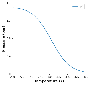
Now we’re ready to solve the actual problem. We’ll start by solving for the equilibrium partial pressure of species C for a large set of temperatures. We’ll use a for loop to run opt.newton or opt.brent many times…
Tset   = np.linspace(200, 400, 100)
pCout1 = np.zeros(len(Tset))

for i in range(0, len(Tset)):
    Tval  = Tset[i]
    obj1d = lambda ex: temp(ex, Tval)
    ans, info = opt.newton(obj1d, 0.999, full_output = True)
    if info.converged == False:
        print('Solver failed to Converge')
        break

    #Workup
    NA0 = 1.0 #mole
    NB0 = 1.0 #mole
    NC0 = 0.0 #moles
    P   = 1.5 #bar

    NA  = NA0 - ans #moles
    NB  = NB0 - ans #moles
    NC  = NC0 + ans #moles
    NT  = NA + NB + NC

    yA  = NA/NT
    yB  = NB/NT
    yC  = NC/NT

    pA  = yA*P
    pB  = yB*P
    pC  = yC*P

    pCout1[i] = pC
plt.figure(1, figsize = (5,5))
plt.plot(Tset, pCout1, label = 'pC')
plt.ylim(0, 1.6)
plt.yticks(np.arange(0, 1.61, 0.4))
plt.xlim(Tset[0], Tset[-1])
plt.ylabel('Pressure (bar)', fontsize = 14)
plt.xlabel('Temperature (K)', fontsize = 14)
plt.legend()
plt.show()
Solution Part 1e#
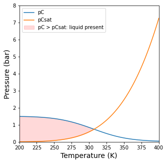
Now let’s compare that to the vapor pressure of species C, which we can evaluate directly from the Clausius-Clapeyron Equation.
Product C has a fairly low vapor pressure, so we are concerned about the formation of a liquid phase in the reactor. The Clausius-Clapeyron equation gives the vapor pressure of component C in units of bar as a function of temperature.
The reactor is initially filled with an equimolar mixture of A and B. The equilibrium constant at T = 298K is K = 9, the reaction is exothermic with \(\Delta H^{\circ} = -11\) kcal/mol, and the system pressure is P = 1.5 bar. Components A and B are not very soluble in liquid C, so you can assume that if a liquid phase forms, it is pure species C (A and B do not condense). The heat of vaporization of component C is \(\Delta {H_{\text{vap}}} = 6\) kcal/mol, and the value of the Clausius-Clapeyron contant is c = 9.53.
def pCsat(T):
    c = 9.53
    DHvap = 6 #kcal/mol
    R = 1.987e-3 #kcal/mol/K
    return np.exp(c - DHvap/R/T)
def pCsat(T):
    c = 9.53
    DHvap = 6 #kcal/mol
    R = 1.987e-3 #kcal/mol/K
    return np.exp(c - DHvap/R/T)
plt.figure(1, figsize = (5,5))
plt.plot(Tset, pCout1, label = 'pC')
plt.plot(Tset, pCsat(Tset), label = 'pCsat')
plt.ylim(0, 8)
plt.yticks(np.arange(0, 8.1, 1))
plt.xlim(Tset[0], Tset[-1])
plt.ylabel('Pressure (bar)', fontsize = 14)
plt.xlabel('Temperature (K)', fontsize = 14)
plt.fill_between(Tset, pCout1, pCsat(Tset), where = pCout1 >= pCsat(Tset), interpolate = True, color = 'red', alpha = 0.15, label = 'pC > pCsat: liquid present')
plt.legend(loc = 'upper left')
plt.show()
Finding the transition temperature#
If you want to solve for the exact temperature where the two curves intersect, there are many ways you can probably do it. Below, I show a modification to our objective function so that it takes two unknowns (ex and Temperature) in a vector argument (var). You’ll note that I added a second constraint equation to the equilibrium problem, which is that pC = pCsat. This will solve for the intersection temperature in the figure above (and the extent at that temperature).
def obj1e(var):
    ex = var[0]
    T  = var[1]

    NA0 = 1.0 #mole
    NB0 = 1.0 #mole
    NC0 = 0.0 #moles
    T0  = 298 #K
    #T   = 400 #K
    P   = 1.5 #bar
    P0  = 1.0 #bar
    DH0 = -11.0 #kcal/mol
    R   = 1.987e-3 #kcal/mol/K

    NA  = NA0 - ex #moles
    NB  = NB0 - ex #moles
    NC  = NC0 + ex #moles
    NT  = NA + NB + NC

    yA  = NA/NT
    yB  = NB/NT
    yC  = NC/NT

    PC  = yC*P

    aA  = yA*P/P0
    aB  = yB*P/P0
    aC  = yC*P/P0

    K0 = 9
    KTHERMO   = K0*np.exp(-DH0/R*(1/T - 1/T0))
    KACTIVITY = aC/aA/aB
    OBJECTIVE1 = KTHERMO - KACTIVITY
    OBJECTIVE2 = PC - pCsat(T)
    return [OBJECTIVE1, OBJECTIVE2]
opt.root(obj1e, [0.5, 300])
    fjac: array([[-0.99541068,  0.09569527],
       [-0.09569527, -0.99541068]])
     fun: array([ 1.11639586e-10, -1.67610370e-12])
 message: 'The solution converged.'
    nfev: 11
     qtf: array([-6.02853354e-08, -4.88374628e-09])
       r: array([14.3419963 ,  0.79060035,  0.09239627])
  status: 1
 success: True
       x: array([  0.66161408, 307.21390082])
Basically, above 307.2K, there is no liquid phase. Below 307.2K, there is a liquid phase.
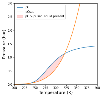
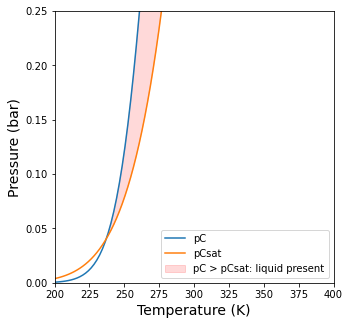
Problem 2
If the reaction is endothermic with \(\Delta H^{\circ} = 11\) kcal/mol, over what temperature range does the reactor contain a liquid phase?
def temp2(ex, T):
    NA0 = 1.0 #mole
    NB0 = 1.0 #mole
    NC0 = 0.0 #moles
    T0  = 298 #K
    #T   = 400 #K
    P   = 1.5 #bar
    P0  = 1.0 #bar
    DH0 = 11.0 #kcal/mol
    R   = 1.987e-3 #kcal/mol/K

    NA  = NA0 - ex #moles
    NB  = NB0 - ex #moles
    NC  = NC0 + ex #moles
    NT  = NA + NB + NC

    yA  = NA/NT
    yB  = NB/NT
    yC  = NC/NT

    aA  = yA*P/P0
    aB  = yB*P/P0
    aC  = yC*P/P0

    K0 = 9
    KTHERMO   = K0*np.exp(-DH0/R*(1/T - 1/T0))
    KACTIVITY = aC/aA/aB
    OBJECTIVE = KTHERMO - KACTIVITY
    return OBJECTIVE
Tset   = np.linspace(200, 400, 100)
pCout2 = np.zeros(len(Tset))

for i in range(0, len(Tset)):
    Tval  = Tset[i]
    obj2a = lambda ex: temp2(ex, Tval)
    ans, info = opt.newton(obj2a, 0.999, full_output = True)
    if info.converged == False:
        print('Solver failed to Converge')
        break

    #Workup
    NA0 = 1.0 #mole
    NB0 = 1.0 #mole
    NC0 = 0.0 #moles
    P   = 1.5 #bar

    NA  = NA0 - ans #moles
    NB  = NB0 - ans #moles
    NC  = NC0 + ans #moles
    NT  = NA + NB + NC

    yA  = NA/NT
    yB  = NB/NT
    yC  = NC/NT

    pA  = yA*P
    pB  = yB*P
    pC  = yC*P

    pCout2[i] = pC
plt.figure(1, figsize = (5,5))
plt.plot(Tset, pCout2, label = 'pC')
plt.plot(Tset, pCsat(Tset), label = 'pCsat')
plt.ylim(0, 3)
plt.yticks(np.arange(0, 3.1, 0.5))
plt.xlim(Tset[0], Tset[-1])
plt.ylabel('Pressure (bar)', fontsize = 14)
plt.xlabel('Temperature (K)', fontsize = 14)
plt.fill_between(Tset, pCout2, pCsat(Tset), where = pCout2 >= pCsat(Tset), interpolate = True, color = 'red', alpha = 0.15, label = 'pC > pCsat: liquid present')
plt.legend(loc = 'upper left')
plt.show()

plt.figure(2, figsize = (5,5))
plt.plot(Tset, pCout2, label = 'pC')
plt.plot(Tset, pCsat(Tset), label = 'pCsat')
plt.ylim(0, 0.25)
plt.yticks(np.arange(0, 0.26, 0.05))
plt.xlim(Tset[0], Tset[-1])
plt.ylabel('Pressure (bar)', fontsize = 14)
plt.xlabel('Temperature (K)', fontsize = 14)
plt.fill_between(Tset, pCout2, pCsat(Tset), where = pCout2 >= pCsat(Tset), interpolate = True, color = 'red', alpha = 0.15, label = 'pC > pCsat: liquid present')
plt.legend(loc = 'lower right')
plt.show()
def obj2b(var):
    ex = var[0]
    T  = var[1]

    NA0 = 1.0 #mole
    NB0 = 1.0 #mole
    NC0 = 0.0 #moles
    T0  = 298 #K
    #T   = 400 #K
    P   = 1.5 #bar
    P0  = 1.0 #bar
    DH0 = 11.0 #kcal/mol
    R   = 1.987e-3 #kcal/mol/K

    NA  = NA0 - ex #moles
    NB  = NB0 - ex #moles
    NC  = NC0 + ex #moles
    NT  = NA + NB + NC

    yA  = NA/NT
    yB  = NB/NT
    yC  = NC/NT

    PC  = yC*P

    aA  = yA*P/P0
    aB  = yB*P/P0
    aC  = yC*P/P0

    K0 = 9
    KTHERMO   = K0*np.exp(-DH0/R*(1/T - 1/T0))
    KACTIVITY = aC/aA/aB
    OBJECTIVE1 = KTHERMO - KACTIVITY
    OBJECTIVE2 = PC - pCsat(T)
    return [OBJECTIVE1, OBJECTIVE2]
opt.root(obj2b, [0.2, 230])
    fjac: array([[-0.92096132,  0.38965402],
       [-0.38965402, -0.92096132]])
     fun: array([ 6.88048230e-12, -9.28743193e-13])
 message: 'The solution converged.'
    nfev: 20
     qtf: array([-4.78581906e-09, -1.25987421e-09])
       r: array([ 2.18306257e+00, -8.58397519e-03, -1.14420384e-03])
  status: 1
 success: True
       x: array([5.25451872e-02, 2.37072654e+02])
There is a liquid phase present between 237.1K and 321.2K. In this region, pC > pCsat, so there will be condensation.