Kinetics X
Contents
Kinetics X#
This lecture considers the analysis of surface reactions (heterogeneous catalysis). We introduce the reaction equilibrium assumption and develop the Langmuir-adsorption model, which has wide usage in catalysis and adsorption phenomena.
import matplotlib.pyplot as plt
import numpy as np
import scipy.optimize as opt
Heterogeneous Catalysis#
When we discuss heterogeneous catalysis, we are generally referring to overall gas- or liquid-phase reactions that occur through a series of intermediate steps on a solid surface. The classic example that we’ve used in this course is that of ammonia synthesis in the Haber-Bosch process.
Ammonia Synthesis#
Overall, that gas-phase reaction is this:
However, what actually is happening is that \(N_2\) and \(H_2\) molecules from the gas phase are dissociating on exposed Fe or Ru atoms on the catalyst surface. An illustration of that basic idea is given below.

So, this is a bit what catalysis looks like on a metal surface. The exposed atoms are “active sites” that facilitate reactions of species that are stable in the gas phase. Things are a little more complicated in a real reactor. The conversion we achieve in a catalytic reactor depends on the number of these “active sites” that are present in the reactor, which ultimately depends on the amount of catalyst surface area inside of the reactor. Bulk metal particles have very low surface area (few active sites per unit area), so, in order to achieve practical levels of fractional conversion, we would have to put a very large and expensive quantity of bulk Ni, Fe, Ru, Pt, etc. inside of our reactor.
Porous materials#
Our usual workaround for this is to use a very high surface area material as a “support.” High surface area materials are generally porous solids. Imagine a sponge with pores that are on the nanometer scale. Frequently these materials have massive surface areas, on the order of 100 - 1000 m\(^2\) per gram. These porous materials allow you to pack a very large surface area into a reasonably sized reactor (because they have so much surface area per unit mass). Pretty much any kind of industrial heterogeneous catalysis we can imagine is actually going to occur on the surface of these porous materials. If it is an acid catalyzed reaction, we would have protons (H\(^+\)) distributed on the surface of these materials. These protons would be our “active sites.” A base catalyst would have electron rich species distributed on the surface (O\(^{2-}\)). If we need a metal catalyst, we would usually “disperse” it onto this high surface area material. Ultimately, this would look like many very small metal nanoparticles (1 - 20 nm) that are stabilized on the high surface area support (something like SiO\(_2\) or Al\(_2\)O\(_3\)).

In this way, we can maximize the metal surface area (by virtue of having very small particles) and so make our catalyst cost effective and practical for use in an industrial reactor.
Packed bed reactors#
For practical reasons, we cannot fill a reactor with nanometer sized particles of high surface area support with catalystic sites on them, which would a) be generally costly and energy intensive to manufacture consistently and b) cause enormous pressure drops in the packed bed. In reality, we are usually working with porous catalyst “pellets” (white spheres in the PBR below) that have macroscale dimensions on the order of centimeters or inches, and where the vast majority of “active sites” are embedded inside of the pores (see gray spheres inside of the inert porous pellet).

This sets up an additional bit of complexity:
Active sites are distributed throughout these inch-scale porous materials (see illustration of packed bed above), and there is no convective flow in their pores…so reacting species, in the course of flowing through the packed bed in the bulk gas phase or liquid phase, have to diffuse through the porous particle, to the active site before they can react. Then, the products have to diffuse away from the active site and back into the bulk flow before we can recover them at the exit of the reactor.
This actually means that you can have multiple phenomena controlling the rate at which the catalyst converts reactants into products. If the rate of diffusion to and from the active sites is very fast (and reaction is relatively slow), then the process is usually controlled by adsorption and reaction on the active sites. If you have very fast reactions (compared to diffusion), then the rate of mass transfer will control the rate at which reactants are converted to products.
If you want to learn more about designing reactors where catalysts operate under conditions of heat or mass transfer, you can take my graduate course (CEN 786). For the rest of this analysis, we will make the following assumption when dealing with surface reactions:
We will assume that rates of heat and mass transfer in the reactor and the catalyst pellet are infinitely fast relative to rates of reaction
This means that the temperature and composition in the bulk fluid are identical to the temperature and composition at the active site inside of the porous pellet, and it makes our analysis much simpler.
Mechanisms of (Heterogeneous) Catalytic Reactions#
Now we’ll focus in on the mechanisms of catalytic reactions. Sticking with ammonia synthesis, we can think of this conceptually as surface active sites facilitating dissociation of N\(_2\) and H\(_2\) to form N- and H- atoms bound to “active sites” on the catalyst surface. The H atoms can add sequentially to N atoms to eventually form ammonia, which desorbs from the surface. We can translate that into a set of elementary steps:
We use a specific notation in these elementary reactions. Species present in the bulk (gas or liquid phase) are written without any specific subscripts. The * symbol represents a vacant active site. And a chemical species with a * as the subscript means that species is bound to the active site (*) on the catalyst surface. When we write rate expressions for these elementary step, we’ll use a slightly different convention than usual.
Rates depend on the concentration of species present in the bulk gas or liquid phase. In this problem, that would be N\(_2\), H\(_2\), and NH\(_3\).
We make the “mean field approximation,” which assumes that surface species are randomly distributed on the surface (they do not segregate into islands, for example) and that their motion on the surface by diffusion is very, very fast relative to reaction rates.
If the mean field approximation holds, rates depend on the fractional coverage of surface species or active sites just as they do concentrations for bulk species. The fractional coverage is defined as the number of surface species or vacant sites divided by the total number of active sites. We use a symol \(\theta_j\) to represent the fractional coverage of the surface species (or vacant surface site).
As an example, if we wanted to write a rate expression for step 1, we note that it involves the dissociation of an N\(_2\) molecule at 2 active sites to form 2 surface bound nitrogen atoms:
And if I wanted to write a rate expression for the third step, we would write:
We’ll work our way back up to the analysis of full mechanisms, but first we will introduce a couple of concepts and simplifications that we frequently use in the analysis of catalytic reactions.
The Langmuir Isotherm#
In almost every catalytic reaction, we have to consider adsorption and desorption of species. There are two types of adsorption: molecular adsorption and dissociative adsorption. We’ll illustrate both types below and see how they work out.
As we do this, notice that desorption is simply adsorption in reverse, so I almost always write these as “adsorption” steps going from left-to-right. You may see that other people write separate “desorption” steps, but they are just adsorption steps written in the right-to-left direction.
Molecular Adsorption#
When a molecule adsorbs on a surface without any bonds breaking, this is usually called molecular adsorption. For example, let’s say we have a molecule like ammonia that adsorbs on a surface without breaking any bonds, we would write that step as we did in step 6 for the HB mechanism of ammonia synthesis.
That is a molecular adsorption step! (Note that the reverse of this step would be described as the molecular desorption of ammonia.) We often represent adsorption steps generically as follows:
Since this is an elementary step, we can write the rate of that reaction using the rules outlined above. It will depend on the bulk concentration of A and on the surface coverage of vacant sites and molecularly adsorbed A:
Molecular adsorption steps tend to be relatively fast. There is no real bond scission occuring, so we usually approximate them as having a 0 activation barrier. This generally means a large rate constant. Often, on the timescales of reactions, fast adsorption processes are actually very nearly at equilibrium. Not always, but frequently we will assume that adsorption steps are at equilibrium. When a reaction is at equilibrium, we know that the rate in the forward direction is exactly the same as the rate in the reverse direction. In other words, the net rate of reaction is zero.
So, if a step is at equilbrium, we would write:
And one could solve this expression for the fractional coverage of species A in terms of the bulk concentration of A and the fractional coverage of vacant sites:
For an elementary step, we know that the ratio of the forward and reverse rate constant is equal to the equilibrium constant for that step, so:
We’ve run into this problem a lot – we have an expression of the coverage of A in terms of something, free (vacant) sites, that are difficult to measure/quantify/control in the laboratory. We would like to know the coverage of A in terms of bulk concentrations and kinetic parameters. But notice, this is the coverage (concentration) of a species bound to the catalyst, and we’ve expressed it as a function of the coverage (concentration) of vacant active sites (free catalyst). We can resolve the coverage of vacant sites using a site balance. For this system, the surface site exists in two states–it is either vacant, or it has species A bound to it, so the site balance for this system is:
It’s still based on the same assumption as usual–that the total number of active sites is constant–but since we’ve expressed their concentrations as fractional coverages, the coverages of all species must always sum to 1. We can substitute the expression for \(\theta_A*\) into the site balance:
And now we’re in familiar territory from our work with enzymatic reactions. We can solve this expression for the fraction of vacant sites:
With that, we can substitute it into the expression for \(\theta_A\) to get the coverage of A in terms of its bulk concentration and an equilibrium constant.
This is the classic Langmuir adsorption isotherm, and it is used frequently to model adsorption processes. We note that it has the following limiting behaviors:
At low concentrations of A (\(C_A \rightarrow 0\)):
In other words, the coverage of A increases with a first order depedence on the concentration of A.
At high concentrations of A (\(C_A \rightarrow \infty\)):
In other words, it is zero order in A. All of the surface sites are saturated with species A, and increasing the concentration of A can’t do anything to increase the coverage of A beyond saturation.
The Difference Between The Equilibrium Assumption and the PSSH#
A lot of students confuse the equilibrium assumption with the pseudo-steady state assumption. Briefly, equilibrium is something we assume about a reaction. Steady state is something we assume about a species. So, if I was making an equilibrium assumption, I would do so on a single reaction as I’ve done above. Whereas I would make a steady state approximation about a species.
Equilibrium
PSSH
These are fundamentally different approximations! It is extremely important to recognize the difference if for no other reason that using equilibrium approximations make it much easier to develop rate expressions for surface reactions. You can use PSSH approximations, but the algebra can quickly become impossible so that there is now way to solve the equations analytically. The point: if you are allowed to make an equilibrium approximation about an elementary step in a surface reaction mechanism, do it. Do not try to use a PSSH because you will get lost in the algebra.
Dissociative Adsorption#
Many molecules–like \(N_2\) and \(H_2\) in our Haber-Bosch example, dissociate (break bonds) when they adsorb on a catalyst surface. In those examples, \(N_2\) forms 2 surface-bound N atoms, and \(H_2\) forms 2 surface-bound H atoms. This type of adsorption is usually called dissociative adsorption. Looking at the dissociative adsorption steps from the HB mechanism, you’ll see it is a bit unique in that it requires 2 vacant active sites–one for each species formed by the bond dissociation event.
The reverse of these steps would be described as the associative desorption of N\(_2\) or H\(_2\). We often represent a dissociative adsorption steps generically as follows:
Since this is an elementary step, we can write the rate of that reaction using our conventions for surface reactions under the mean field approximation. It will depend on the bulk concentration of B\(_2\), the surface coverage of vacant sites (*), and the surface coverage of B atoms:
Notice: Because this step involves two vacant sites and two surface atoms, when we write the rate expression, it will depend on the square of their coverages.
Dissociative adsorption is a bit more kinetically difficult than molecular adsorption (we do have to break a bond here), so they may have an activation barrier. Even still, they are usually small barriers relative to surface reactions. So even dissociative adsorption steps are usually fast compared to surface reactions. As in the case of molecular adsorption, we frequently assume that dissociative adsorption steps are at equilibrium (although this is a bad approximation for the specific example of N\(_2\), which I’ve unfortunately chosen as an illustration case here).
If we can assume a dissociative adsorption step is at equilibrium, then we say the net rate of that step is zero as we did with molecular adsorption:
Keeping in mind that a convenient solution strategy for these mechanistic analyses is to solve for the coverage of a bound species as a function of vacant site coverage, we solve for \(\theta_B\):
And we replace the rate constant ratio for a single elementary step with an equilibrium constant:
And we’re in a familiar spot where we have the coverage of the bound species expressed as a linear function of bulk concentration, an equilibrium constant, and the free sites. We resolve the free site coverage with a site balance as usual. Again, we’ll assume the catalyst site can exist in two states. It can either be vacant (*) or it can have a B adsorbed at it (B\(_*\)). Since the sum of all fractional coverages is 1:
We then substitute the expression for \(\theta_B*\) into the site balance:
Again, notice that we’ve approached the problem in such a way that all terms on the right hand side of our site balance have a linear dependence on vacant site coverage, so this is easy to solve for \(\theta_*\):
With that, we can substitute it into the expression for \(\theta_B\) to get the coverage of B in terms of its bulk concentration and an equilibrium constant.
This is the Langmuir isotherm for dissociative adsorption! It is definitely a result worth knowing. We can also consider its behavior at high and low concentrations of the adsorbing species:
At low concentrations of B\(_2\) (\(C_{B_2} \rightarrow 0\)):
In other words, the coverage of B increases with a half-order depedence on the concentration of B\(_2\).
At high concentrations of B\(_2\) (\(C_{B_2} \rightarrow \infty\)):
In other words, it is zero order in B\(_2\). All of the surface sites are saturated with species B, and increasing the concentration of B\(_2\) can’t do anything to increase the coverage of B beyond saturation.
Distinguishing Between Molecular and Dissociative adsorption#
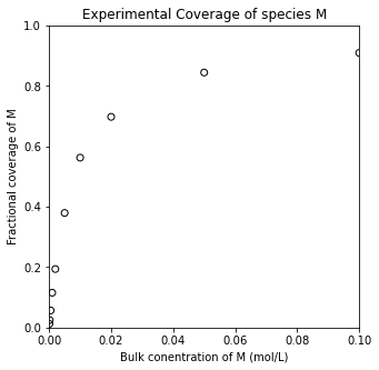
There are a number of ways that we can do this, but all of them involve running experiments where we vary the bulk concentration (or, in the gas phase, partial pressure) of the adsorbing species, we allow the adsorption step to equilibrate, and we measure the quantity of species adsorbed on the catalyst surface. There are various methods of doing this. The most common is to quantify the decrease in bulk species and assume that any species lost from the bulk have adsorbed on the surface. Another strategy can be to use a quartz crystal microbalance to actually detect the change in mass of the catalyst as species adsorb on the surface. Finally, if you are careful to calibrate an infrared spectrometer using one of the above methods, you can use something like FTIR to quantify the amount of species adsorbed on a surface. Once we do this, we will have a set of surface coverages at equilibrium with various gas- or liquid-phase concentrations, and we would work through our usual tools of data analysis and reconciliation of proposed models with experimental measurements.
For example, you could perform nonlinear regression to fit the associative and dissociative adsorption models to data and determine which best fits your data set. An example is shown below.
CM_exp     = np.array([0.0001, 0.0002, 0.0005, 0.001, 0.002, 0.005, 0.01, 0.02, 0.05, 0.1]) #mol/L
thetaM_exp = np.array([0.01231471, 0.02450419, 0.05662556, 0.11536265, 0.19374295, 0.37952173, 0.56262205, 0.69767484, 0.84451735, 0.90949091])

plt.figure(1, figsize = (5, 5))
plt.scatter(CM_exp, thetaM_exp, color = 'none', edgecolor = 'black')
plt.xlim(0, 0.1)
plt.ylim(0, 1)
plt.title('Experimental Coverage of species M')
plt.xlabel('Bulk conentration of M (mol/L)')
plt.ylabel('Fractional coverage of M')
plt.show()
Next we’ll fit molecular and dissociative adsorption models to see if one clearly fits better than the other. We’ll do that using the following models for the fractional coverage of M:
Molecular Adsorption
Dissociative Adsorption
I’m not doing anything new here: I’m just fitting two nonlinear models to our data by generating objective functions and minimizing the residual sum of squares (by varying the adsorption constant).
def obj_molecular(par):
    KM = par
    CM = CM_exp

    thetaM_mod = KM*CM/(1 + KM*CM)

    SSE = np.sum((thetaM_exp - thetaM_mod)**2)
    return SSE

def obj_dissociative(par):
    KM = par
    CM = CM_exp

    thetaM_mod = (KM*CM)**(1/2)/(1 + (KM*CM)**(1/2))

    SSE = np.sum((thetaM_exp - thetaM_mod)**2)
    return SSE

ans_mol = opt.minimize_scalar(obj_molecular)
ans_dis = opt.minimize_scalar(obj_dissociative)

KM_mol = ans_mol.x
KM_dis = ans_dis.x

SSE_mol = ans_mol.fun
SSE_dis = ans_dis.fun

SST     = np.sum((thetaM_exp - np.mean(thetaM_exp))**2)

R2_mol  = 1 - SSE_mol/SST
R2_dis  = 1 - SSE_dis/SST
And then we can plot the models with our optimum results against our experimental data to assess goodness of fit.
CMfine     = np.linspace(0, 0.1, 100)
thetaM_mol = lambda CM: (KM_mol*CM)/(1 + KM_mol*CM)
thetaM_dis = lambda CM: (KM_dis*CM)**(1/2)/(1 + (KM_dis*CM)**(1/2))

print(f'For molecular adsorption   , we get KM = {KM_mol:3.0f} L/mol, SSE = {SSE_mol:3.2E}, and R2 = {R2_mol:3.3f}')
print(f'For dissociative adsorption, we get KM = {KM_dis:3.0f} L/mol, SSE = {SSE_dis:3.2E}, and R2 = {R2_dis:3.3f}')

plt.figure(1, figsize = (5, 5))
plt.scatter(CM_exp, thetaM_exp, color = 'none', edgecolor = 'black', label = 'experimental data')
plt.plot(CMfine, thetaM_mol(CMfine), color = 'black', linestyle = 'dashed', linewidth = 1, label = 'Molecular Adsorption Model')
plt.plot(CMfine, thetaM_dis(CMfine), color = 'red', linestyle = 'dashed', linewidth = 1, label = 'Dissociative Adsorption Model')
plt.xlim(0, 0.1)
plt.ylim(0, 1)
plt.title('Experimental Coverage of species M')
plt.xlabel('Bulk conentration of M (mol/L)')
plt.ylabel('Fractional coverage of M')
plt.show()
For molecular adsorption   , we get KM = 121 L/mol, SSE = 7.78E-04, and R2 = 0.999
For dissociative adsorption, we get KM = 105 L/mol, SSE = 1.24E-01, and R2 = 0.887
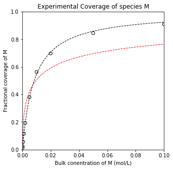
You can visually determine that the molecular adsorption model provides a much better fit to this data set. This is also borne out in quantative metrics like the SSE and the R2 value.
Linearization of Isotherms#
It is also useful to be able to linearize these models, which is relatively easy to do. We see that both coverage expressions are monomial functions divided by a polynomial, so we can linearize these models by inversion.
Molecular Adsorption
Dissociative Adsorption
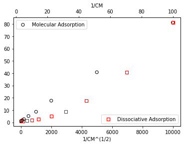
If we have molecular adsorption, plotting coverage vs. inverse concentration should give a straight line. If we have dissociative adsorption, we’ll see a straight line if we plot coverage vs. inverse square root of concentration. This is illustrated below for the data set above (which we already determined is well-described by molecular adsorption). You can see clearly that the data plotted against inverse concentration is linear, which agrees with the molecular adsorption model.
fig, ax1     = plt.subplots()
ax2          = ax1.twiny()
molecular    = ax1.scatter(1/CM_exp, 1/thetaM_exp, marker = 'o', color = 'none', edgecolor = 'black', label = 'Molecular Adsorption')
dissociative = ax2.scatter(1/CM_exp**(1/2), 1/thetaM_exp, marker = 's', color = 'none', edgecolor = 'red', label = 'Dissociative Adsorption')

ax1.set_xlabel('1/CM^(1/2)')
ax2.set_xlabel('1/CM')
ax2.set_ylabel('1/thetaM')

ax1.legend(loc = 'upper left')
ax2.legend(loc = 'lower right')
plt.show()