
Jupyter and Python
Contents
Jupyter and Python#
Everyone should have completed the review materials (Supplements 01 - 07) by this point. Today, we will be getting familiar with the Jupyter Environment and basic Python. Here is an overview of the topics:
Base Python vs. Numpy (lists vs. arrays)
1D arrays, columns, rows, and matrices
Basic math operators in Python
Functions
For Loops, While Loops
Element-wise operations (broadcasting) vs. matrix operations
Logical values and conditional statements
Graphing
We’ll go through some some practice exercises in the cells below.
Lists and Numpy Arrays#
If we’re going to work in Python, we need to discuss the differences between lists and numpy arrays. It is easy to confuse these two types of data structures since they look similar, and we create them in similar ways. But they have important differences. We will usually want to work with numpy arrays in this course, but I want to communicate why they are a bit more convenient. To do that, we need to discuss lists first.
Lists#
When working with data, functions, and various types of analysis, we generally need to be able to store sets or collections of values instead of just scalars. In the base Python environment, the default type of collection is a list.
Making a List#
If you are familiar with Matlab’s environment, creating a list is very similar to creating an array in Matlab. For example, if we wanted to create a list containing the integers 1 to 5, we would do so as follows:
L1 = [1, 2, 3, 4, 5]
L1 = [1, 2, 3, 4, 5]
whos
Variable   Type    Data/Info
----------------------------
L1         list    n=5
L1[3]
4
dir(L1)
['__add__',
 '__class__',
 '__class_getitem__',
 '__contains__',
 '__delattr__',
 '__delitem__',
 '__dir__',
 '__doc__',
 '__eq__',
 '__format__',
 '__ge__',
 '__getattribute__',
 '__getitem__',
 '__gt__',
 '__hash__',
 '__iadd__',
 '__imul__',
 '__init__',
 '__init_subclass__',
 '__iter__',
 '__le__',
 '__len__',
 '__lt__',
 '__mul__',
 '__ne__',
 '__new__',
 '__reduce__',
 '__reduce_ex__',
 '__repr__',
 '__reversed__',
 '__rmul__',
 '__setattr__',
 '__setitem__',
 '__sizeof__',
 '__str__',
 '__subclasshook__',
 'append',
 'clear',
 'copy',
 'count',
 'extend',
 'index',
 'insert',
 'pop',
 'remove',
 'reverse',
 'sort']
L1.reverse()
L1
[5, 4, 3, 2, 1]
The print command#
We can display the contents of that list and the length of that list. We’ll also display the type.
print(L1)
print(len(L1))
print(type(L1))
print(L1)
print(len(L1))
print(type(L1))
[5, 4, 3, 2, 1]
5
<class 'list'>
Despite appearances, lists are not rows, columns, or matrices#
This looks like a row vector compared to what we are probably used to from Matlab, but it has very different properties. Technically, it is a 1 dimensional object (it only has a length associated with it), whereas rows, columns, and matrices are 2D objects (they have both row and column dimensions).
Let’s say we wanted to store a “2D” set of information in lists; we would do so by constructing a list of lists:
L2 = [[1, 2, 3, 4, 5], [6, 7, 8, 9, 10]]
L2 = [[1, 2, 3, 4, 5], [6, 7, 8, 9, 10]]
If we print that list, we find it looks like a matrix:
print(L2)
print(L2)
[[1, 2, 3, 4, 5], [6, 7, 8, 9, 10]]
However, if we ask for the length of that list, we find that it is only 2 elements long:
len(L2)
len(L2)
2
It is not a 2x5 matrix, and if we tried to index it like a matrix (row, column), we get an error:
L2[1,1]
L2[1,1]
---------------------------------------------------------------------------
TypeError                                 Traceback (most recent call last)
~\AppData\Local\Temp\ipykernel_18968\76180332.py in <cell line: 1>()
----> 1 L2[1,1]

TypeError: list indices must be integers or slices, not tuple
If we wanted to access information in that list, we have to remember that it is not a matrix, but a list of lists…so if I wanted to recall the number 5, for example, from L2, that is not indexed as:
L2[0,4] #5th column in first row of L2
As you might do in Matlab; rather, it is indexed as:
L2[0][4] #5th element in first list of L2
L2[0][4]
5
Creating large lists with the range command#
If we want to create a large list, such as the full set of integers between 1 and 50, we generally won’t type it out. Instead, we’ll pass the range() function into the list() constructor. The basic syntax of range is:
range(start, stop+1, step size)
So for this example:
L = list(range(1, 51, 1))
L = list(range(1, 51, 1))
print(L)
[1, 2, 3, 4, 5, 6, 7, 8, 9, 10, 11, 12, 13, 14, 15, 16, 17, 18, 19, 20, 21, 22, 23, 24, 25, 26, 27, 28, 29, 30, 31, 32, 33, 34, 35, 36, 37, 38, 39, 40, 41, 42, 43, 44, 45, 46, 47, 48, 49, 50]
Numpy Arrays#
If we want a matrix like environment (and we’ll see some reasons for this below), this is best handled in Python using numpy arrays. This is not in base Pyton – we have to import the numpy package to gain access to numpy arrays.
import numpy as np
import numpy as np
Making a numpy array#
We create numpy arrays as in the following example. Here, we create a 1D numpy array that contains the integers 1 to 5 (similar to the list above).
A1 = np.array([1, 2, 3, 4, 5]) #equivalent to np.array(L1)
The way numpy arrays are created is that we actually pass a list into the array constructor. It is going to be very important to remember this when we create 2D arrays (similar to a matrix) or higher dimensional arrays.
A1 = np.array([1, 2, 3, 4, 5])
whos
Variable   Type       Data/Info
-------------------------------
A1         ndarray    5: 5 elems, type `int32`, 20 bytes
L          list       n=50
L1         list       n=5
L2         list       n=2
np         module     <module 'numpy' from 'C:\<...>ges\\numpy\\__init__.py'>
A1[0]
1
Examining the numpy array#
Let’s print that array and check it’s properties and dimensions; we’ll compare it to the analogous list and consider some of the differences.
print(A1)
print(len(A1))
print(type(A1))
print(L1)
print(len(L1))
print(type(L1))
print()
print(A1)
print(len(A1))
print(type(A1))
[5, 4, 3, 2, 1]
5
<class 'list'>

[1 2 3 4 5]
5
<class 'numpy.ndarray'>
Numpy arrays have a lot of useful features built into them#
Looking at numpy arrays, we can see that they have a lot more attributes than lists do; many of these are useful in mathematics, statistics, and engineering. We can also use them to assess the size and shape of our arrays.
print(A1.max())
print(A1.min())
print(A1.size)
print(A1.shape)
print(A1.ndim)
dir(A1)
['T',
 '__abs__',
 '__add__',
 '__and__',
 '__array__',
 '__array_finalize__',
 '__array_function__',
 '__array_interface__',
 '__array_prepare__',
 '__array_priority__',
 '__array_struct__',
 '__array_ufunc__',
 '__array_wrap__',
 '__bool__',
 '__class__',
 '__complex__',
 '__contains__',
 '__copy__',
 '__deepcopy__',
 '__delattr__',
 '__delitem__',
 '__dir__',
 '__divmod__',
 '__doc__',
 '__eq__',
 '__float__',
 '__floordiv__',
 '__format__',
 '__ge__',
 '__getattribute__',
 '__getitem__',
 '__gt__',
 '__hash__',
 '__iadd__',
 '__iand__',
 '__ifloordiv__',
 '__ilshift__',
 '__imatmul__',
 '__imod__',
 '__imul__',
 '__index__',
 '__init__',
 '__init_subclass__',
 '__int__',
 '__invert__',
 '__ior__',
 '__ipow__',
 '__irshift__',
 '__isub__',
 '__iter__',
 '__itruediv__',
 '__ixor__',
 '__le__',
 '__len__',
 '__lshift__',
 '__lt__',
 '__matmul__',
 '__mod__',
 '__mul__',
 '__ne__',
 '__neg__',
 '__new__',
 '__or__',
 '__pos__',
 '__pow__',
 '__radd__',
 '__rand__',
 '__rdivmod__',
 '__reduce__',
 '__reduce_ex__',
 '__repr__',
 '__rfloordiv__',
 '__rlshift__',
 '__rmatmul__',
 '__rmod__',
 '__rmul__',
 '__ror__',
 '__rpow__',
 '__rrshift__',
 '__rshift__',
 '__rsub__',
 '__rtruediv__',
 '__rxor__',
 '__setattr__',
 '__setitem__',
 '__setstate__',
 '__sizeof__',
 '__str__',
 '__sub__',
 '__subclasshook__',
 '__truediv__',
 '__xor__',
 'all',
 'any',
 'argmax',
 'argmin',
 'argpartition',
 'argsort',
 'astype',
 'base',
 'byteswap',
 'choose',
 'clip',
 'compress',
 'conj',
 'conjugate',
 'copy',
 'ctypes',
 'cumprod',
 'cumsum',
 'data',
 'diagonal',
 'dot',
 'dtype',
 'dump',
 'dumps',
 'fill',
 'flags',
 'flat',
 'flatten',
 'getfield',
 'imag',
 'item',
 'itemset',
 'itemsize',
 'max',
 'mean',
 'min',
 'nbytes',
 'ndim',
 'newbyteorder',
 'nonzero',
 'partition',
 'prod',
 'ptp',
 'put',
 'ravel',
 'real',
 'repeat',
 'reshape',
 'resize',
 'round',
 'searchsorted',
 'setfield',
 'setflags',
 'shape',
 'size',
 'sort',
 'squeeze',
 'std',
 'strides',
 'sum',
 'swapaxes',
 'take',
 'tobytes',
 'tofile',
 'tolist',
 'tostring',
 'trace',
 'transpose',
 'var',
 'view']
2D and nD Arrays#
With numpy arrays, we can actually create 2D or higher dimensional structures (3D, 4D, etc.) We’ll mostly stick with 1D and 2D in CEN 587. For example, let’s recreate that list of lists above as a numpy array using the array constructor.
The key thing to remember when you are creating a 2D array is that you still use the basic np.array() constructor syntax:
np.array([])
But every row in the array should be entered into the np.array() constructor as a list.
A2 = np.array([[1, 2, 3, 4, 5], [6, 7, 8, 9, 10]]) #equivalent to np.array(L2)
If you look closely at this, you’ll see that the first “element” in that array is the list [1, 2, 3, 4, 5], and the second element is the list [6, 7, 8, 9, 10]. These “elements” in a numpy array correspond to rows in a matrix, so when you’re creating a matrix, you enter each row as a separate list. Each list should be separated by a comma.
A2 = np.array([[1, 2, 3, 4, 5], [6, 7, 8, 9, 10]])
Now we’ll look at that array and some of its associated properties and dimensions:
print(A2)
print(len(A2))
print(type(A2))
print(A2.size)
print(A2.shape)
print(A2.ndim)
print(L2)
print(len(L2))
print(type(L2))
print()

print(A2)
print(len(A2))
print(type(A2))
print(A2.size)
print(A2.shape)
print(A2.ndim)
[[1, 2, 3, 4, 5], [6, 7, 8, 9, 10]]
2
<class 'list'>

[[ 1  2  3  4  5]
 [ 6  7  8  9 10]]
2
<class 'numpy.ndarray'>
10
(2, 5)
2
Indexing in numpy arrays#
With a numpy array, we have the option of indexing it as we would a matrix using [row, column] indexing, so, with this numpy array, if I wanted to grab the fifth column in the first row, I can do so as:
A2[0,4] #5th column in first row
or as I would with a list:
A2[0][4] #5th element in first element
So: a numpy array has size, shape, and index options that are similar to what we are probably used to with Matlab matrices. Lists do not translate directly to matrix format.
print(A2[0,4])  #5th column in first row
print(A2[0][4]) #5th element in first element
5
5
1D arrays vs. Rows and Columns#
If you are coming from a Matlab background, you are used to thinking of “vectors” of numbers or entries as either rows (horizontal set of values) or columns (vertical set of values). It is important to remember that rows and columns are 2-dimensional structures – they both have a length (number of rows) and width (number of columns) associated with them.
Specifically, a column is m rows x 1 column…and a row is 1 row x n columns. These are 2D structures and they have the corresponding shapes associated with them.
Whereas Matlab creates rows and columns by default using brackets [], spaces, or semicolons, Python is slightly different.
Let’s go back to our original set of integers from 1 to 5. If I create a numpy array as follows:
A1 = np.array([1, 2, 3, 4, 5])
And print its values as well as its dimensions and shape:
print(A1)
print(A1.shape)
print(A1.ndim)
We will find that it is a true 1 dimensional structure. It is a “line” of values, and it is neither a row or column in that it has no horizontal or vertical orientation associated with it. This is what the somewhat strange notation (5,) communicates to us. There is no 2nd dimension.
A1 = np.array([1, 2, 3, 4, 5])
print(A1)
print(A1.ndim)
print(A1.shape)
[1 2 3 4 5]
1
(5,)
Usually, we’ll be fine working with 1D arrays. They will typically behave either as a row or a column depending on context (if we need them to). If we ever specifically need to create a row or a column, we have to deliberately create a 2D array. For example, recreating that 1D array as a row looks like this:
R1 = np.array([[1, 2, 3, 4, 5]])
Look at it closely and you’ll see that I’m still passing a list into the np.array() constructor with [], and the first element in that list is another list enclosed in an additional set of []. This is how you create 2D arrays in Python with numpy arrays.
R1 = np.array([[1, 2, 3, 4, 5]])
And we’ll print important aspects as usual:
print(R1)
print(R1.shape)
print(R1.ndim)
Now, you see that we have a true row of shape (1, 5), i.e., 1 row and 5 columns.
print(R1)
print(R1.shape)
print(R1.ndim)
[[1 2 3 4 5]]
(1, 5)
2
In contrast, if we really need a column, we would have to create it as follows (again, as a 2D array):
C1 = np.array([[1], [2], [3], [4], [5]])
Again, you’ll notice that I’m passing a list into an np.array() constructor using a set of values enclosed in []. In this case, each element in that list is also a separate list enclosed in brackets [], and I’ve created several rows by entering every value as its own list separated by commas. With numpy arrays, each new “list” separated by commas creates a new row, so in this example, we’ve made a column with 5 rows.
C1 = np.array([[1], [2], [3], [4], [5]])
And we display outputs:
print(C1)
print(C1.ndim)
print(C1.shape)
Which reveal that this is actually a column.
print(C1)
print(C1.ndim)
print(C1.shape)
[[1]
 [2]
 [3]
 [4]
 [5]]
2
(5, 1)
More often than not, we only need to work with 1D arrays and matrices, but it is important to understand what these shapes mean. I found myself initially very confused by 1D arrays when I switched from Matlab to Python, so I thought the explanation was worthwhile. If I run into an occasion where we actually need a row or a column, we’ll discuss it. Most of the time, 1D numpy arrays will suffice where we think we need a row or a column.
Tools for creating large numpy arrays#
We want to create a 1D numpy array, A, that has the numbers 1 through 50 in it. We can do this in at least three ways:
Write out the integers 1 to 50 separated by commas in an np.array constructor (not recommended).
A = np.array([1, 2, 3, 4, 5, ... , 48, 49, 50])
Use np.arange() (good option, can be flaky with non-integer step sizes).
A = np.arange(start, stop+1, step size) #same as np.array(range(start, stop+1, step size) for int
Use np.linspace() to construct the array (returns floats; usually what we want; probably most useful option).
A = np.linspace(start, stop, number of elements in collection)
A = np.linspace(1, 50, 50)
#A = np.arange(1, 51, 1) #Roughly equivalent to np.linspace(1, 50, 50)
#A = np.array(range(1, 51, 1)) #equivalent to np.arange(1, 51, 1)
#A = np.array(L) #effectively the same as np.arange(1, 51, 1) since we have list L created above
Lists vs. arrays in practice (math!)#
As a simple demonstration, let’s just try a few basic math operations on our 50 element array, A, and our 50 element list, L.
A + 5
L + 5
A*5
L*5
A**2  #A squared
L**2  #L squared
# A + 5
# L + 5
# A*5
# L*5
# A**2  #A squared
# L**2  #L squared
Now we’ll create a second 1D array, B, that has the numbers 2 through 100 in increments of 2.
B = np.linspace(2, 100, 50)
Element-wise calculations are easy with arrays#
Let’s take advange of element-wise operations (broadcasting) in numpy arrays to:
Multiply each element in A by each element in B
Raise each element in A to the third power
Find the exponential of the cube root of each element in A
Divide each element in B by each element in A
Each should give a 50 element vector (why?)
A*B
A**3
np.exp(A**(1/3))
B/A
array([2., 2., 2., 2., 2., 2., 2., 2., 2., 2., 2., 2., 2., 2., 2., 2., 2.,
       2., 2., 2., 2., 2., 2., 2., 2., 2., 2., 2., 2., 2., 2., 2., 2., 2.,
       2., 2., 2., 2., 2., 2., 2., 2., 2., 2., 2., 2., 2., 2., 2., 2.])
Basic Matrix Operations#
Now we’ll get a look at Matrix operations in Python. To perform a matrix operation on something, we usually need a 2D array, so we’ll use our rows and columns for this.
Look at the difference between C1 and its transpose. #use np.transpose(C1) or C1.T
Look at the difference between R1 and its transpose. #use np.transpose(R1) or R1.T
Multiply C1 by C1\(^T\) - this should give a 5x5 array (why?) #use C1@C.T
Multiply R1 by R1\(^T\) - this should give a 1x1 array (why?) #use R1@R.T
print(C1, '\n') #'\n' adds a new line, effectively this is a "return" command
print(C1.T, '\n')
print(R1, '\n')
print(R1.T, '\n')
print(C1@C1.T, '\n')
print(R1@R1.T)
[[1]
 [2]
 [3]
 [4]
 [5]]

[[1 2 3 4 5]]

[[1 2 3 4 5]]

[[1]
 [2]
 [3]
 [4]
 [5]]

[[ 1  2  3  4  5]
 [ 2  4  6  8 10]
 [ 3  6  9 12 15]
 [ 4  8 12 16 20]
 [ 5 10 15 20 25]]

[[55]]
Introducing np.zeros and np.ones#
You can use np.zeros to create an array of zeros; here, we’ll create a 3x5 array of zeros.
np.zeros(shape) #Shape should be a tuple (immutable list, give or take).
(3, 5); a list [3, 5]; or an nd array using numpy, np.array([3, 5]). Usually I use a tuple for this.
Similarly, you can use np.ones to create an array of ones.
D = np.zeros((3,5))
O = np.ones((3,5))

print(D, '\n\n', O) #'\n\n' is a string that is basically saying press enter twice
[[0. 0. 0. 0. 0.]
 [0. 0. 0. 0. 0.]
 [0. 0. 0. 0. 0.]]

 [[1. 1. 1. 1. 1.]
 [1. 1. 1. 1. 1.]
 [1. 1. 1. 1. 1.]]
D.size
D.shape
rows, cols = D.shape #note that D.shape returns a tuple, i.e., "multiple returns".
Basic for loops#
Use a for loop to print all of the values in C1
Use a for loop to fill in the values of D such that each element in D is equal to the sum of it’s (i,j) index pair.
#A simple for loop that runs through all the values in C1

for value in C1:
    print(value)
[1]
[2]
[3]
[4]
[5]
#A for loop with some bells and whistles.  It runs over two indices, i and j, in a nested loop.
#It prints information on each pass and also does a calculation and stores the result in D

for i in range(0, rows):
    print(f'\nThis is pass number {i+1} through the outer loop')
    for j in range(0, cols):
        print(f'i = {i}, j = {j}, i+j = {i+j}')
        D[i,j] = i + j
print('\n', D)
This is pass number 1 through the outer loop
i = 0, j = 0, i+j = 0
i = 0, j = 1, i+j = 1
i = 0, j = 2, i+j = 2
i = 0, j = 3, i+j = 3
i = 0, j = 4, i+j = 4

This is pass number 2 through the outer loop
i = 1, j = 0, i+j = 1
i = 1, j = 1, i+j = 2
i = 1, j = 2, i+j = 3
i = 1, j = 3, i+j = 4
i = 1, j = 4, i+j = 5

This is pass number 3 through the outer loop
i = 2, j = 0, i+j = 2
i = 2, j = 1, i+j = 3
i = 2, j = 2, i+j = 4
i = 2, j = 3, i+j = 5
i = 2, j = 4, i+j = 6

 [[0. 1. 2. 3. 4.]
 [1. 2. 3. 4. 5.]
 [2. 3. 4. 5. 6.]]
Finding the determinant (matrix must be square)#
Find the determinant of:
E = np.array([[1,7,9],[21,-4,17],[-6,22,6]])
print(E)
np.linalg.det(E)
[[ 1  7  9]
 [21 -4 17]
 [-6 22  6]]
1948.0
Matrix inverse in numpy#
Find the inverse of \(E\)
np.linalg.inv(E)
array([[-0.20431211,  0.08008214,  0.07956879],
       [-0.11704312,  0.03080082,  0.08829569],
       [ 0.224846  , -0.03285421, -0.0775154 ]])
Functions and graphing#
This section covers some basic function definitions and plotting tools using pyplot
Long form function definition#
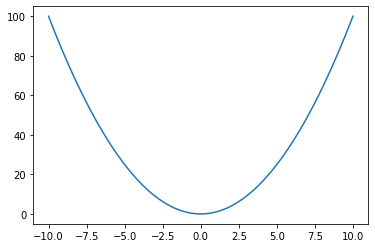
Let’s create a function that accepts one input using a conventional function declaration.
Plot y(x) on the domain \(x = [-10, 10]\); add labels for x and y axis.
def y(x):
    y = x**2
    return y
y(10)
100
x = np.linspace(-10, 10, 100)
import matplotlib.pyplot as plt
plt.plot(x, y(x))
[<matplotlib.lines.Line2D at 0x26202f18b50>]
A multivariate function using a lambda function definition#
Now we’ll create a function that accepts two inputs; here, we’ll use an inline or anonymous function syntax.
What is the value of f at x = 10, y = 7?
f = lambda x,y: np.sin(x) + np.cos(y)
f(10, 7)
0.20988114345393483
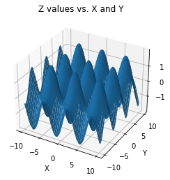
3D plotting syntax#
Create a 3D plot of the surface on the domain \(x = [-10, 10]\) and \(y = [-10,10]\); add labels and title.
fig, ax = plt.subplots(subplot_kw={"projection": "3d"})

#Data
x = np.linspace(-10, 10, 100)
y = np.linspace(-10, 10, 100)
X, Y = np.meshgrid(x, y) #we're making a surface plot, so we create a grid of (x,y) pairs
Z = f(X,Y)  #generate the Z data on the meshgrid (X,Y) by evaluating f at each XY pair.

#Plot the surface.
surf = ax.plot_surface(X, Y, Z)
plt.xlabel('X')
plt.ylabel('Y')
plt.title('Z values vs. X and Y')
plt.show()
Multiple arguments, and multiple returns#
Now, let’s create a function, \(g(x,t)\), that accepts multiple inputs and returns multiple outputs - value(s) for y and values for z as a function of \((x,t)\). We can look at this as a system of functions
Calculate the values of y and z at x = 10, t = 7.
def g1(x,t):
    y = x**2*t
    z = x*np.cos(t)
    return y, z #this will return a tuple of (y, z) by default.
                #A tuple is declared with and indicated by parentheses ().
                #A tuple is an immutable array.
print(g1(10, 7), '\n')

y, z = g1(10, 7) #when I have multiple returns, I can bind them to individual variables this way.
print(f'y = {y}, z = {z}')
(700, 7.539022543433046)

y = 700, z = 7.539022543433046
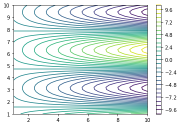
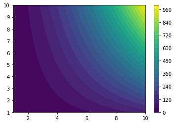
How about a contour plot?#
Use the function \(g(x,t)\) to generate values for both \(y\) and \(z\) on the domain \(x = [0, 10]\) and \(t = [0, 10]\); create a contour plot for \(y(x,t)\) and \(z(x,t)\).
x = np.linspace(1,10,50)
t = np.linspace(1,10,50)
[X, T] = np.meshgrid(x,t)
Y, Z = g(X,T)

plt.figure()
plt.contour(X, T, Z, levels = 25)
plt.colorbar()

plt.figure()
plt.contourf(X, T, Y, levels = 25)
plt.colorbar()

plt.show()
x = np.linspace(1,10,50)
t = np.linspace(1,10,50)
[X, T] = np.meshgrid(x,t)
Y, Z = g(X,T)

plt.figure()
plt.contour(X, T, Z, levels = 25)
plt.colorbar()

plt.figure()
plt.contourf(X, T, Y, levels = 25)
plt.colorbar()

plt.show()
You can create very complex functions…#
Let’s add some complexity to that same function \(g(x,t)\). It still will take two inputs \((x,t)\), but let’s add to the outputs. Let’s have it return an 3x3 matrix of zeros; a 5x5 matrix of ones; and a character array that says IT’S A TRAP!
Print the 5 outputs for the \((x,t)\) input pair \((1,1)\).
def g2(x,t):
    y = x**2*t
    z = x*np.cos(t)
    m1 = np.zeros((3,3))
    m2 = np.ones((5,5))
    s1 = "IT'S A TRAP"
    return y, z, m1, m2, s1

display(g2(1,1))

y, z, m1, m2, s1 = g(1,1)

print(y, '\n')
print(z, '\n')
print(m1, '\n')
print(m2, '\n')
print(s1, '\n')
(1,
 0.5403023058681398,
 array([[0., 0., 0.],
        [0., 0., 0.],
        [0., 0., 0.]]),
 array([[1., 1., 1., 1., 1.],
        [1., 1., 1., 1., 1.],
        [1., 1., 1., 1., 1.],
        [1., 1., 1., 1., 1.],
        [1., 1., 1., 1., 1.]]),
 "IT'S A TRAP")
1

0.5403023058681398

[[0. 0. 0.]
 [0. 0. 0.]
 [0. 0. 0.]]

[[1. 1. 1. 1. 1.]
 [1. 1. 1. 1. 1.]
 [1. 1. 1. 1. 1.]
 [1. 1. 1. 1. 1.]
 [1. 1. 1. 1. 1.]]

IT'S A TRAP