Energy Balances IV

This lecture continues with Energy Balance example problems.

import matplotlib.pyplot as plt
import numpy as np
import scipy.optimize as opt
from scipy.integrate import solve_ivp
from scipy.interpolate import interp1d

Energy Balances on Ideal Reactors

Batch Reactor

The material balance for species j in a well-mixed batch reactor is:

\[\frac{dN_j}{dt} = R_jV\]

In cases where we have either an incompressible fluid or our reactor operates at constant pressure, the energy balance on a batch reactor is:

\[\sum_j N_j \bar{C}_{p,j} \frac{dT}{dt} = -\sum_i \Delta H_{i} r_i V + \dot{Q}\]

A few notation conventions: the bar over a property here means it is an intensive molar property for a species and it has units of “per mole”. \(\dot{Q}\) is the rate of heat exhange with the surroundings. It is given by:

\[\dot{Q} = UA(T_a - T)\]

CSTR

The material balance for species j in a CSTR is:

\[\frac{dN_j}{dt} = F_{jf} - F_j + R_jV\]

If we have an incompressible fluid or a reactor operating at constant pressure, the energy balance on a CSTR is:

\[\sum_j N_j \bar{C}_{p,j} \frac{dT}{dt} = -\sum_i \Delta H_{i} r_i V + \sum_j F_{jf}(\bar{H}_{jf} - \bar{H}_j) + \dot{Q}\]

The rate of heat exchange is the same as in a batch reactor:

\[\dot{Q} = UA(T_a - T)\]

PFR

The material balance for species j in a PFR is:

\[\frac{dF_j}{dV} = R_j\]

If we have an ideal gas or a reactor operating without a pressure drop, the energy balance for a PFR is:

\[\sum_j F_j \bar{C}_{p,j} \frac{dT}{dV} = -\sum_i \Delta H_{i} r_i + \dot{q}\]

For a PFR, we express the rate of heat transfer per unit volume, and it has a symbol \(\dot{q}\):

\[\dot{q} = Ua(T_a - T)\]

Example Problem 01

(Fogler, Example 12.5)

This example considers non-isothermal operation of a PFR with multiple reactions. Specifically, the following two gas phase reactions:

(172)\[\begin{align} A &\longrightarrow B\\ 2A &\longrightarrow C \end{align}\]

Where both reactions have elementary rate laws. Pure A (\(C_{Af} = 0.1\) moles per liter) is fed to the reactor at a rate of 100 moles per second and a temperature of 150\(^\circ\)C. We additionally are provided the following information:

(173)\[\begin{align} k_{10} &= 10 \ \textrm{s}^{-1} \\ k_{20} &= 0.045 \ \textrm{L} \ \textrm{mol}^{-1} \ \textrm{s}^{-1} \\ \frac{E_{A1}}{R} &= 4000 \ \textrm{K} \\ \frac{E_{A2}}{R} &= 9000 \ \textrm{K} \\ \Delta H_{10} &= -20000 \ \textrm{J} \ \textrm{mol}^{-1} \\ \Delta H_{20} &= -120000 \ \textrm{J} \ \textrm{mol}^{-1} \\ C_{PA} &= 90 \ \textrm{J} \ \textrm{mol}^{-1} \ \textrm{K}^{-1} \\ C_{PB} &= 90 \ \textrm{J} \ \textrm{mol}^{-1} \ \textrm{K}^{-1} \\ C_{PC} &= 180 \ \textrm{J} \ \textrm{mol}^{-1} \ \textrm{K}^{-1} \\ Ua &= 4000 \ \textrm{J} \ \textrm{L}^{-1} \ \textrm{s}^{-1} \ \textrm{K}^{-1} \\ T_{a} &= 100^\circ\textrm{C} \end{align}\]

Note: reported rate constants were measured at 300K

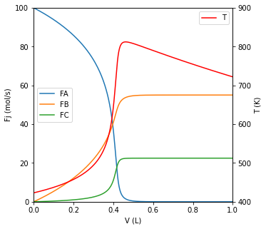
Assume this PFR has a total volume \(V = 1.0 \ \mathrm{L}\) ; plot the molar flowrates of all species as well as the temperature as a function of reactor volume.

Solution to Example Problem 01

We are asked to plot the flowrate of each species and the temperature as a function of reactor volume. Clearly, we need to write material and energy balances.

For this system, we have 3 species, so we write 3 material balances:

(174)\[\begin{align} \frac{dF_A}{dV} = R_A \\ \frac{dF_B}{dV} = R_B \\ \frac{dF_C}{dV} = R_C \\ \end{align}\]

We also write an energy balance on the reactor:

\[\frac{dT}{dV} = \frac{-\sum_i \Delta H_i r_i + \dot{q}}{\sum_j F_j \bar{C}_{p,j}}\]

Now we just specify everything on the right hand side of those ODEs in terms of constants, the 4 dependent variables, or volume (our independent variable).

Production rates:

(175)\[\begin{align} R_A &= -r_1 - 2r_2 \\ R_B &= r_1 \\ R_C &= r_2 \\ \end{align}\]

Rate expressions:

(176)\[\begin{align} r_1 &= k_1C_A\\ r_2 &= k_2{C_A}^2 \end{align}\]

Concentration of A:

\[C_A = \frac{F_A}{Q}\]

Use an equation of state to define Q:

\[Q = \frac{F_TRT}{P}\]

Where R and P are both constant and expressed in appropriate units, and T is a state variable in the ODE system. We define total molar flowrate in terms of individual species:

\[F_T = F_A + F_B + F_C\]

Next, we need to define our rate constants as functions of temperature; we do so using a van’t Hoff type expression (since we are given rate constants measured at a specific temperature).

(177)\[\begin{align} k_1 &= k_{10}\exp\left[-\frac{E_{A1}}{R}\left(\frac{1}{T} - \frac{1}{T_0}\right)\right] \\ k_2 &= k_{20}\exp\left[-\frac{E_{A2}}{R}\left(\frac{1}{T} - \frac{1}{T_0}\right)\right] \\ \end{align}\]

We also need to know the heats of reaction at the reaction temperature in order to complete the material balance. We know that, generally:

\[\Delta H(T) = \Delta H^\circ + \int_{T_0}^{T} \Delta C_p dT\]

For both of these reactions, we find that \(\Delta C_p = 0\), so we conclude that heats of reaction are temperature independent here.

This is a non-isothermal reactor with heat exchange; we calculate the rate of heat exchange per unit volume (\(\dot{q}\)) as follows:

\[\dot{q} = Ua(T_a - T)\]

Where the temperature of the heat exchange fluid (\(T_a\)) and the product of the heat transfer coefficient (U) and the surface area-per-volume (a) are given in the problem statement.

That should be it. ODE system is fully specified and can be solved.

def P01(V, var):
   
    #Fixed values from problem statement
    Tf   = 150 + 273 #K
    Cf   = 0.1 #mol/L
    R    = 0.08206 #L*atm/mol/K
    Pf   = Cf*R*Tf #atm
    P    = Pf #atm
    k10  = 10 #1/s
    k20  = 0.045 #L/mol/s
    DH1  = -20000 #J/mol
    DH2  = -120000 #J/mol
    EAR1 = 4000 #K
    EAR2 = 9000 #K
    CPA  = 90 #J/mol/K
    CPB  = 90 #J/mol/K
    CPC  = 180 #J/mol/K
    Ua   = 4000 #J/L/K/s
    Ta   = 100+273 #K
    T0   = 300 #K
    
    #Quantities changing as a function of reactor volume.
    FA = var[0]
    FB = var[1]
    FC = var[2]
    T  = var[3]
    FT = FA + FB + FC #mol/s
    Q  = FT*R*T/P     #L/s
    
    CA = FA/Q         #mol/L
    
    k1 = k10*np.exp(-EAR1*(1/T - 1/T0)) #1/s
    k2 = k20*np.exp(-EAR2*(1/T - 1/T0)) #L/mol/s
    
    r1 = k1*CA     #mol/L/s
    r2 = k2*CA**2  #mol/L/s
    
    RA = -r1 - 2*r2  #mol/L/s
    RB =  r1         #mol/L/s
    RC =  r2         #mol/L/s
    
    qdot = Ua*(Ta - T) #J/L/s
    
    DT = (-1*(DH1*r1 + DH2*r2) + qdot)/(FA*CPA + FB*CPB + FC*CPC)
    
    D1 = RA
    D2 = RB
    D3 = RC
    D4 = DT
    
    return [D1, D2, D3, D4]

FAf  = 100 #mol/s
FBf  = 0
FCf  = 0
Tf   = 150 + 273 #K
var0 = [FAf, FBf, FCf, Tf]
vspan = (0.0, 1.0) #L
ans   = solve_ivp(P01, vspan, var0, atol = 1e-10, rtol = 1e-10)

V             = ans.t
FA, FB, FC, T = ans.y

fig1, ax1 = plt.subplots(figsize = (5, 5))
ax2 = ax1.twinx()
ax1.plot(V, FA, label = 'FA')
ax1.plot(V, FB, label = 'FB')
ax1.plot(V, FC, label = 'FC')
ax2.plot(V, T,  color = 'red', label = 'T')

ax1.set_xlim(0.0, 1.0)
ax1.set_ylim(0, 100)
ax2.set_ylim(400, 900) 

ax1.set_xlabel('V (L)')
ax1.set_ylabel('Fj (mol/s)')
ax2.set_ylabel('T (K)')

ax1.legend(loc = 'center left')
ax2.legend(loc = 'upper right')

<matplotlib.legend.Legend at 0x205c7a7c910>