Material Balances XII
Material Balances XII#
This lecture covers reactor sequencing using Levenspiel Plots
import numpy as np
import matplotlib.pyplot as plt
import scipy.optimize as opt
from scipy.integrate import quadrature, solve_ivp
from scipy.interpolate import interp1d
from math import ceil, floor
Flow Reactors in Series
Before we begin, let’s just state that we’ll still apply the general simplifying assumptions we’ve been using to this point, i.e., all parameters (k, CAf, FAf, Q, etc.) all have a numerical value of 1, and units are always such that they give reactor volumes in Liters. We’ll also assume that density, temperature, pressure, volumetric flowrates, etc. are constant in this sequence of reactors. Mostly, this is so that we can make the following simplification, which just makes it less messy to solve problems:
Let’s now consider carrying out a reaction in a set of flow reactors in sequence instead of in a single flow reactor:

We can express the molar flowrate at any point in this sequence in terms of the feed molar flowrate to the process, \(F_{A0}\) and the overall conversion achieved at a particular point in the sequence. In other words:
Let’s recall our generic balance on a single CSTR solved for Volume:
And the same for a generic balance on a single PFR solved for Volume:
Looking at those, we can remind ourselves that the size of the reactor will scale directly with the quantity of species converted in that reactor. The more stuff that we convert in the reactor, generally, the larger it needs to be. Let’s generalize the concept of the quantity of stuff that gets converted in the reactor. For example, you could look at Reactor 1 and say that the quantity of A consumed in Reactor 1 is given by \(F_{A0} - F_{A1}\). We can express that quantity in terms of conversion using the results above:
We can simplify this significantly:
Similarly, if we wanted to express the quantity of A converted across the second reactor in terms of the process feed, \(F_{A0}\), and fractional conversions, we would write:
Which simplifies to:
We can see a pattern emerging – for the “nth” flow reactor in a series, we can quantify the amoutn of reactant converted in that reactor as:
Consider the nth reactor
Now, let’s think conceputally about that nth reactor in the sequence (see figure below):

If we were to write a CSTR balance on the nth reactor, we’d find:
We can solve this for the volume of the nth reactor:
And recognizing that, for this simple \(A \longrightarrow B\) reaction, \(R_{A_n} = -r_n\):
Where, importantly, the rate of reaction is determined by the concentration inside of the nth reactor, which is equal to the concentration in the exit stream from the nth reactor. We can replace the difference in molar flowrates in the numerator with the fractional conversion expression from above to get:
In order to actually solve this, we have to specify a rate law. We’ll again use the generic power law kinetics that we’ve been assuming so far:
With that, I can write a generic function to solve for the nth CSTR in a sequence. All I need to do is give it the fractional conversion into that CSTR, \(X_{A_{(n-1)}}\), the fractional conversion out of that CSTR, \(X_{A_n}\), and the reaction order \(\alpha\).
def VCSTR(XAin, XAout, alpha):
    FAf = 1 #mol/min
    Qf  = 1 #mol/min
    CAf = 1 #mol/L
    k   = 1 #1/min
    CA  = CAf*(1 - XAout)
    r   = k*CA**alpha
    V   = FAf*(XAout - XAin)/r
    return V
Now that we have this, we’ll use it to calculate the CSTR volume required to take the system from 0% to 90% conversion across a single reactor; we find that it is 9.0L as usual.
VC  = VCSTR(0.0, 0.90, 1)
print(f'{VC:3.2f}')
9.00
Now let’s do something different. Let’s set up two CSTRs in series and have them achieve 90% conversion together. For simplicity, we’ll have the first CSTR achieve 45% conversion (it takes the system from 0% conversion to 45% conversion), and we’ll have the second CSTR achieve the remainder (it takes the system from 45% conversion to 90% conversion).
VC1 = VCSTR(0.0, 0.45, 1)
VC2 = VCSTR(0.45, 0.90, 1)
VCT = VC1 + VC2
print(f'{VC:3.2f}')
print(f'{VC1:3.2f}')
print(f'{VC2:3.2f}')
print(f'{VCT:3.2f}')
9.00
0.82
4.50
5.32
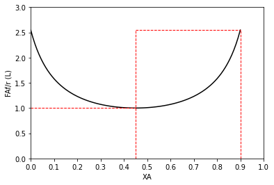
That’s interesting! The first CSTR requires 0.82L of volume to go to 45% conversion, and the second reactor requires 4.50L to go from 45% to 90% conversion. If we add those together, that’s 5.32L of total CSTR volume if we divide the system into 2 CSTRs, each accomplishing half of the required conversion. In contrast, if we try to do this in a single CSTR, it costs us 9.0L of reactor volume.
Why is that so? It has to do with the fact that CSTR are assumed to be perfectly mixed, and they operate entirely at the exit conversion. If we try to achive 90% conversion in a single reactor, that entire reactor operates at 90% conversion, where the concentration of A is 10% of its feed value. For a positive order, that means the rate is actually quite low throughout the reactor, so it takes 9.0L of volume.
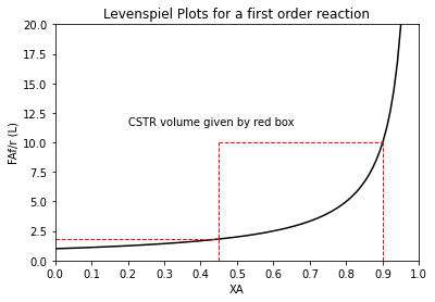
In contrast, if we divide this into two reactors, the first one operates at 45% conversion, so the concentration in that reactor is 0.55CAf. For a positive order reaction, this means the rate in that first reactor is realtively high compared to a CSTR operating at 90% conversion (0.1CAf). So that reactor converts 45% of the feed at a relatively high reaction rate; hence the relatively small size.
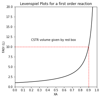
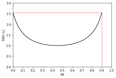
The second reactor is operating at 90% conversion (0.1CAf), which means a very low reaction rate for a positive order reaction; however, it now only has to convert 45% of the feed, so the “stuff” converted at that low rate is less, and we have a smaller second reactor than the 9.0L we’d need to convert 90% of the feed in a single CSTR. This is very easy to see on a Levenspiel Plot.
def LEV(XA, alpha):
    k   = 1 #units to vary with reaction order so that r = mol/L/min
    CAf = 1 #mol/L
    FAf = 1 #mol/min
    CA  = CAf*(1 - XA)
    r   = k*CA**alpha
    return FAf/r
order = 1
XAset = np.linspace(0, 0.95, 100)
plt.figure(1, figsize = (5, 5))
plt.plot(XAset, LEV(XAset, order), color = 'black')
plt.vlines(0.9, 0, 10, linestyle = 'dashed', color = 'red', linewidth = 1)
plt.hlines(LEV(0.9, order), 0.0, 0.9, linestyle = 'dashed', color = 'red', linewidth = 1)
plt.annotate('CSTR volume given by red box', (0.2, 11.5))
plt.title('Levenspiel Plots for a first order reaction')
plt.ylabel('FAf/r (L)')
plt.xlabel('XA')
plt.xlim(0,1)
plt.ylim(0,20)
plt.xticks(np.linspace(0, 1, 11))
plt.show()
order = 1
XAset = np.linspace(0, 0.95, 100)
plt.plot(XAset, LEV(XAset, order), color = 'black')
plt.vlines(0.9, 0, 10, linestyle = 'dashed', color = 'red', linewidth = 1)
plt.hlines(LEV(0.9, order), 0.45, 0.9, linestyle = 'dashed', color = 'red', linewidth = 1)
plt.vlines(0.45, 0, 10, linestyle = 'dashed', color = 'red', linewidth = 1)
plt.hlines(LEV(0.45, order), 0, 0.45, linestyle = 'dashed', color = 'red', linewidth = 1)
plt.annotate('CSTR volume given by red box', (0.2, 11.5))
plt.title('Levenspiel Plots for a first order reaction')
plt.ylabel('FAf/r (L)')
plt.xlabel('XA')
plt.xlim(0,1)
plt.ylim(0,20)
plt.xticks(np.linspace(0, 1, 11))
plt.show()
Now let’s consider the implications for a series of PFRs. Recall that if we solve a PFR balance for volume in a single reactor, we get the following result:our general balance is given by the following expression:
This balance actually allows for continuous variation in rate as a function of fractional conversion…so we really don’t need to modify it much to consider the volume of the nth reactor. All we do to change it is to realize that calculating the volume of a PFR in the above expression requires us to integrate from the conversion at the inlet of that reactor (it is zero for a single reactor) to the exit of that reactor (it is whatever conversion we’re trying to achieve for a single reactor). If we want to think about the nth reactor in a series of PFRs, we would just account for this by generalizing the limits of integration. I’m also changing the \(F_{A,f}\) to an \(F_{A0}\) to reflect that we’re specifying the fractional conversion at points (n-1) and n relative to point 0, i.e., which is typically the inlet to the process.
Once we have a rate law, we can solve this either analytically, with an ODE solver, or, in this case, since it is just a definite integral, using gaussian quadrature. I’ll take the last option here since it is easy for me to generalize for any reaction order, and I can keep my rate law generic, i.e.,:
def VPFR(XAin, XAout, alpha):
    FAf = 1 #mol/min
    Qf  = 1 #mol/min
    CAf = 1 #mol/L
    k   = 1 #1/min

    intfun   = lambda X: FAf/k/CAf/(1 - X)**alpha
    vol, err = quadrature(intfun, XAin, XAout)
    return vol
Now that this is done, we’ll calculate the PFR volume required to take the system from 0% conversion to 90% conversion in a single reactor:
VP  = VPFR(0.0, 0.90, 1)
print(f'{VP:3.2f}L')
2.30L
We find that it is 2.30L, just like we did in the last lecture where we developed a solution for a single PFR. Now let’s divide it into 2 PFRs in sequence. The first one will take the system from 0% to 45% conversion, and the second one will take the system from 45% to 90% conversion.
VP1 = VPFR(0.0, 0.45, 1)
VP2 = VPFR(0.45, 0.90, 1)
VPT = VP1 + VP2
print(f'{VP:3.2f}L')
print(f'{VP1:3.2f}L')
print(f'{VP2:3.2f}L')
print(f'{VPT:3.2f}L')
2.30L
0.60L
1.70L
2.30L
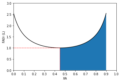
Huh. We see that each reactor is smaller, but that makes sense because they are accomplishing less conversion compared to the single, 2.30L reactor that is achieving 90% conversion in one shot. But if we add them up, we get an identical result to what we got for a single PFR. Again, the reason for this is evident if you look at a Levenspiel plot:
order = 1
XAset = np.linspace(0, 0.95, 100)
XAPFR = np.linspace(0, 0.90, 100)
plt.plot(XAset, LEV(XAset, order), color = 'black')
plt.fill_between(XAPFR, LEV(XAPFR, order))
plt.vlines(0.9, 0, 10, linestyle = 'dashed', color = 'red', linewidth = 1)
plt.hlines(LEV(0.9, order), 0.45, 0.9, linestyle = 'dashed', color = 'red', linewidth = 1)
plt.vlines(0.45, 0, 10, linestyle = 'dashed', color = 'red', linewidth = 1)
plt.hlines(LEV(0.45, order), 0, 0.45, linestyle = 'dashed', color = 'red', linewidth = 1)
plt.annotate('CSTR volume given by red box', (0.2, 11.5))
plt.annotate('PFR volume given by shaded area', (0.35, 0.5))
plt.title(f'Levenspiel Plots for a {order} order reaction')
plt.ylabel('FAf/r (L)')
plt.xlabel('XA')
plt.xlim(0,1)
plt.ylim(0, ceil(max(LEV(XAset, order))))
plt.xticks(np.linspace(0, 1, 11))
plt.show()
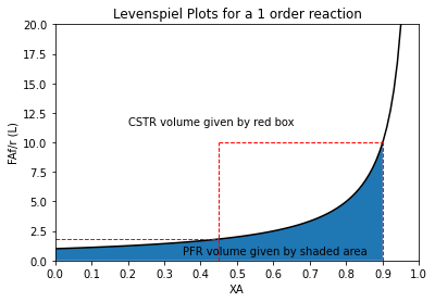
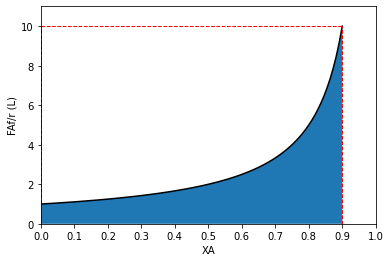
Since PFRs take the system from inlet conditions to exit conditions in a series of differential steps, the volume of the PFR is given by the area under the Levenspiel curve, and there is absolutely no difference if we use a single PFR or if we divide the system into two PFRs.
order = 1
XAset = np.linspace(0, 0.90, 100)
plt.plot(XAset, LEV(XAset, order), color = 'black')
plt.fill_between(XAPFR, LEV(XAPFR, order))

XAMAX = max(XAset)
NREAC = 1
XAVAL = np.linspace(0, XAMAX, NREAC+1)
for i in range(0, len(XAVAL)-1):
    plt.vlines(XAVAL[i], 0, LEV(XAVAL[i+1], order), linestyle = 'dashed', color = 'red', linewidth = 1)
    plt.vlines(XAVAL[i+1], 0, LEV(XAVAL[i+1], order), linestyle = 'dashed', color = 'red', linewidth = 1)
    plt.hlines(LEV(XAVAL[i+1], order), XAVAL[i], XAVAL[i+1], linestyle = 'dashed', color = 'red', linewidth = 1)
plt.ylabel('FAf/r (L)')
plt.xlabel('XA')
plt.xlim(0,1)
plt.ylim(0, ceil(max(LEV(XAset, order))))
plt.xticks(np.linspace(0, 1, 11))
plt.show()
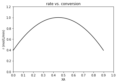
Now let’s consider why these concepts might be useful. Below, I create a Levenspiel plot based on an arbitrary rate law that I have made up entirely so that the rate is parabolic and has a maximum value at around 45% conversion or so. This is not a completely contrived example, by the way. This is actually very commonly encountered when we run exothermic reactions in adiabatic reactors. The reactor increases in temperature due to the heat released by reaction, and this increases the magnitude of the rate constant and accelerates the reaction. Eventually, the concentration of A decreases to the point where it negates the effect of an increasing rate constant, and the reaction begins to slow down again (with increasing conversion). I am mimicking this scenario with this example.
def rmod(XA):
k = 1 #units to vary with reaction order so that r = mol/L/min
CAf = 1 #mol/L
FAf = 1 #mol/min
r = 1 - 3*(XA - 0.45)**2
return r
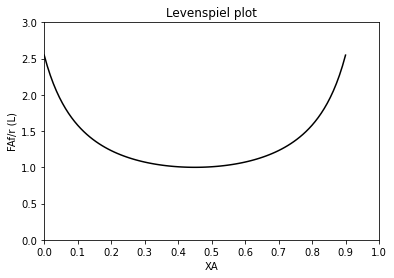
def LEVmod(XA):
k = 1 #units to vary with reaction order so that r = mol/L/min
CAf = 1 #mol/L
FAf = 1 #mol/min
r = 1 - 3*(XA - 0.45)**2
return FAf/r
XAset  = np.linspace(0, 0.90, 100)
XAPFR1 = np.linspace(0.45, 0.9, 100)
XAPFR2 = np.linspace(0.0, 0.45, 100)
plt.figure(1)
plt.plot(XAset, rmod(XAset), color = 'black')
plt.title('rate vs. conversion')
plt.ylabel('r (mol/L/min)')
plt.xlabel('XA')
plt.xlim(0, 1)
plt.ylim(0, ceil(max(rmod(XAset)))*1.2)
plt.xticks(np.linspace(0, 1, 11))

plt.figure(2)
plt.plot(XAset, LEVmod(XAset), color = 'black')
plt.title('Levenspiel plot')
plt.ylabel('FAf/r (L)')
plt.xlabel('XA')
plt.xlim(0,1)
plt.ylim(0, ceil(max(LEVmod(XAset))))
plt.xticks(np.linspace(0, 1, 11))

plt.show()
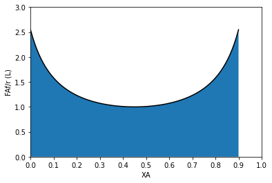
#Use for a single PFR
plt.plot(XAset, LEVmod(XAset), color = 'black')
plt.fill_between(XAset, LEVmod(XAset))
plt.ylabel('FAf/r (L)')
plt.xlabel('XA')
plt.xlim(0,1)
plt.ylim(0, ceil(max(LEVmod(XAset))))
plt.xticks(np.linspace(0, 1, 11))
plt.show()
#Use for a single CSTR
plt.plot(XAset, LEVmod(XAset), color = 'black')
plt.vlines(0.9, 0, LEVmod(0.9), linestyle = 'dashed', color = 'red', linewidth = 1)
plt.hlines(LEVmod(0.9), 0.00, 0.9, linestyle = 'dashed', color = 'red', linewidth = 1)
plt.ylabel('FAf/r (L)')
plt.xlabel('XA')
plt.xlim(0,1)
plt.ylim(0, ceil(max(LEVmod(XAset))))
plt.xticks(np.linspace(0, 1, 11))
plt.show()
#Use for 2 CSTRs in series
plt.plot(XAset, LEVmod(XAset), color = 'black')
plt.vlines(0.9, 0, LEVmod(0.9), linestyle = 'dashed', color = 'red', linewidth = 1)
plt.vlines(0.45, 0, LEVmod(0.9), linestyle = 'dashed', color = 'red', linewidth = 1)
plt.hlines(LEVmod(0.9), 0.45, 0.9, linestyle = 'dashed', color = 'red', linewidth = 1)
plt.hlines(LEVmod(0.45), 0.00, 0.45, linestyle = 'dashed', color = 'red', linewidth = 1)
plt.ylabel('FAf/r (L)')
plt.xlabel('XA')
plt.xlim(0,1)
plt.ylim(0, ceil(max(LEVmod(XAset))))
plt.xticks(np.linspace(0, 1, 11))
plt.show()
#Use for a PFR before a CSTR
plt.plot(XAset, LEVmod(XAset), color = 'black')
plt.vlines(0.9, 0, LEVmod(0.9), linestyle = 'dashed', color = 'red', linewidth = 1)
plt.vlines(0.45, 0, LEVmod(0.9), linestyle = 'dashed', color = 'red', linewidth = 1)
plt.fill_between(XAPFR2, LEVmod(XAPFR2))
plt.hlines(LEVmod(0.9), 0.45, 0.90, linestyle = 'dashed', color = 'red', linewidth = 1)
plt.ylabel('FAf/r (L)')
plt.xlabel('XA')
plt.xlim(0,1)
plt.ylim(0, ceil(max(LEVmod(XAset))))
plt.xticks(np.linspace(0, 1, 11))
plt.show()
#Use for a CSTR before a PFR
plt.plot(XAset, LEVmod(XAset), color = 'black')
plt.vlines(0.45, 0, LEVmod(0.45), linestyle = 'dashed', color = 'red', linewidth = 1)
plt.fill_between(XAPFR1, LEVmod(XAPFR1))
plt.hlines(LEVmod(0.45), 0.00, 0.45, linestyle = 'dashed', color = 'red', linewidth = 1)
plt.ylabel('FAf/r (L)')
plt.xlabel('XA')
plt.xlim(0,1)
plt.ylim(0, ceil(max(LEVmod(XAset))))
plt.xticks(np.linspace(0, 1, 11))
plt.show()