
Kinetics VIII
Contents
Kinetics VIII#
This lecture introduces catalytic reactions. We develop strategies for the analysis of mechanisms catalyzed by enzymes.
import matplotlib.pyplot as plt
import numpy as np
Catalytic Reactions#
There are many, many cases where reactions of interest will not occur at appreciable rates at temperatures and/or pressures that are industrially feasible. Classically, for non-catalytic reactions, you really only have two handles for increasing reaction rate: increasing temperature and increasing concentration. There are practical limits to doing so. These include materials of construction (they may not be able to withstand very high temperatures or pressures); capital cost (it is expensive to construct reactors that can withstand high temperatures and pressures); cost of energy (you generally have to pay in energy costs to run reactions at high temperatures); cost of ancillary equipment (adding a high pressure pump or compressor is expensive; and selectivity reasons (generally, as temperatures increase, more reactions become kinetically accessible, and you lose your ability to control selectivity).
Or just more generally: we know that the cost of a process scales inversely with the rate at which that process occurs. Slow reactions require long batch times or very large flow reactors, so we are frequently interested in running reactions at maximum rate without incurring the difficulties associated with trying to increase reaction rates thermally (by heating). This is where catalysts come in.

Our basic idea of a chemical reaction is that it goes from a rectant state to a product state along some reaction coordinate. The energetic change between reactant state and product state is our energy change of reaction (this applies for any thermodynamic state function: enthalpy, entropy, free energy are most useful in reactions and reactor design). As usual, these quantities determine the equilibrium constant for the reaction, which tells us how far the reaction goes at equilibrium. We also expect that as the reactant transforms into the product along that reaction coordinate, it will generally go through a transition state, which is usually a higher energy species than either the reactant or the product. The energy change associated with forming the transition state is called an “activation barrier,” and we can think of enthalpies of activation, entropies of activation, and free energies of activation. These quantities determine our rate constant for the reaction, which generally communicates how fast the reaction occurs. In order to increase the rate of the reaction, it would be desireable to reduce the barrier associated with forming the transition state.
Generally speaking, a catalyst functions by providing an alternate path between the reactant state and the product state. It does this by coordinating to (loosely, binding with) reactants and products. This induces new types of strain or changes the electron density in key functional groups, which makes it easier to break or to form chemical bonds. One important thing to note is that the catalyst does not affect the reactant state or the product state. These are species present in bulk gas or liquid phase. Whether or not we use a catalyst, the \(N_2\), \(H_2\), and \(N\!H_3\) species present in Ammonia synthesis are the same. Since enthalpies, entropies, and free energies are thermodynamic state functions, this means that a catalyst does not affect the overall energetics of the reaction that we observe in the laboratory. If a reaction is thermodyanmically unfavorable, a catalyst does not change this.
A catalyst does provide a different path between the reactant state and the product state, however. Ideally, this new path will proceed through a lower energy transition state that is generally easier to form. The energetics of forming the transition state determine the rate constant for the reaction, so a catalyst will typically increase the rate of the reaction by virtue of allowing that reaction to proceed through a transition state that is easier to form.
In other words, a catalyst does not change the equilibrium constant for an overall reaction, and it does not make the overall reaction any more or less favorable. A catalyst will increase the rate of reaction, so it increases how quickly that system gets to equilibrium.
Mechanisms of Catalytic Reactions#
The above picture regarding a catalyst decreasing a barrier is conceptually useful; however, just like all reactions, catalytic reactions occur through a series of elementary steps, each with their own characteristic activation barriers (rate constants) and energy changes of reaction (equilibrium constants). These elementary steps will be different than those in the non-catalytic pathway. If we have designed a good catalyst, the net result is that the catalytic mechanism is more kinetically favorable than the non-catalytic mechanism. But it is important to remember that reactions almost always occur through a series of elementary steps, not as a single, overall step that converts reactants into products.
A more complete picture#
Most of us have a basic understanding of catalysis, we’ve probably heard that a catalyst accelerates a reaction but is not itself changed by a reaction. This is true at the macroscopic, observable scale that we work on in the laboratory. A more correct description is that, in the course of the catalytic mechanism, the catalyst is changed substantially as it interacts with the reactant and facilitates its conversion into the product. However, at the conclusion of the catalytic cycle, the product of the reaction disengages from the catalyst, and it is regenerated to its original form so that it can then interact with another reactant molecule and start the cycle over.
Types of Catalytic Reactions#
Broadly speaking, we will consider a few categories of catalytic reactions:
Homogeneous catalysis: In these examples, the catalyst, reactant, product, and all intermediates and transition states are present in a single phase.
Heterogeneous catalysis: In these examples, at least one of the catalyst, reactant, product, intermediates, and/or transition states exist in a second phase.
Biocatalysis: These reactions use an enzyme to facilitate a reaction. They can be either homogeneous (enzyme in solution) or heterogeneous (enzyme immobilized on a support).
We’ll actually start with Biocatalysis because it follows naturally from our consideration of non-catalytic reactions using a Pseudo-steady state approximation.
Enzyme-catalyzed Reactions#
Enzymes are biological molecules comprised of proteins/amino acid and various co-factors, such as metals or metal ions, that are coordinated to the protein. Enzymes are known for their specificity. They are extremely selective in their binding and the types of reactions they will facilitate. Basically, their structure/composition have been optimized over millinea by evolutionary processes, so they tend to be very efficient at catalyzing a specific process.
On the positive side, they operate at low temperatures, they are usually very efficient, and they are extremely selective.
On the negative side, they are biological molecules (proteins) whose function depends on the specific way they are folded. Usually that optimal configuration is only attained in physiological conditions; for example, at approximately 30\(^\circ\)C, near neutral pH, and in aqueous solution. They are extremely sensitive to their environment, so changes in temperature, pH, or the presence of high concentrations of organic molecules can cause enzymes to denature and lose their catalytic function. For this reason they tend to work very well, but only within a limited operating window, which limits our ability to tune their performance in a specific system. Generally speaking, with enzyme catalysts, we will be limited to working in:
Aqueous media
pH of 4 - 9
T of 27\(^\circ\)C to 70\(^\circ\)C
That said, for reactions involving delicate and reactive substrates (like sugars and other biological molecules), enzymes can be very effective, and they are used in many relevant industrial processes. The most prominent example is the production of high fructose corn syrup from starch using amylase and xylose isomerase enzymes. Amylase allows one to very selectively hydrolyse starches into glucose monomers, and xylose isomerase allows one to isomerize glucose into fructose, hence producing “high fructose corn syrup” (note that corn has almost no fructose in it inherently).
Models of Enzyme Catalysis#
The first step in an enzyme catalyzed reaction is that the enzyme (E) will bind to the substrate (S). There are two classic models of enzyme binding:
Lock and Key Model
Induced Fit Model
The latter is more generally accepted because enzymes, being large, flexible molecules that respond to their environment, are much more likely to alter their local structure slightly to bind a substrate than they are to have a rigid pocket that is perfectly matched to the substrate. Regardless, the basic idea is that the enzyme will bind with the substrate. This will then initiate a set of elementary reactions that convert the bound substrate into the product, which ultimately disengages from the enzyme. As such, the Enzyme is returned to its original state at the completion of the catalytic cycle, so we say that it facilitates the conversion of substrate into product without itself being consumed by the reaction.
The most basic mechanism for Enzyme catalysis is the classic Michaelis-Menten model. Conceptually, it says that the enzyme binds the substrate, converting it into a reactive enzyme-substrate complex. This intial binding step is assumed to be reversible. This enzyme substrate complex is then converted into the reaction product. In a classic, baseline Michaelis-Menten model, we assume that the product does not bind at all with the enzyme and so is released immediately upon its formation to irreversibly form the reaction product and a free enzyme. We can write this as an overall reaction and as a set of elementary steps:
Overall
Mechanism
Importantly, we can see that if we add these two elementary steps, it gives us the overall reaction stoichiometry. This is a fundamental requirement – if our reaction mechanism cannot reproduce the overall stoichiometry, then it is incorrect or incomplete in some way.
Analysis
Looking at the overall reaction stoichiometry, we see that the overall rate of reaction is equal to the rate of consumption of substrate (S), and it is equal to the rate of formation of the product (P). We choose to write an overall rate expression based on the rate of product formation.
Now we look at the elementary steps; we can evaluate the production rate of P as usual. It only appears as a product in step 2, so \(R_P = r_2\), which means:
Now we expand the rate expression for step two:
This tells us that the rate of reaction has a first order dependence on the concentration of the enzyme-substrate complex. Unfortunately, this isn’t particularly useful as we will have a difficult time measuring, quantifying, predicting, controlling, etc. the concentration of the enzyme substrate complex. Usually, the enzyme is present in trace amounts relative to the substrate, so we can approximately treat the enzyme-substrate complex as a “reactive intermediate” and apply the Pseudo-steady state approximation. Again, this says that the net production rate of the reactive intermediate is zero:
We can then expand the rate expressions:
My goal, as usual, is to write the concentration of the enzyme-substrate complex in terms of bulk species, like the substrate concentration. Technically, I usually have trouble quantifying the free enzyme concentration [E] since it is going to be present in trace quantities, and it is unclear how much of it is free [E] and how much is bound with the substrate [ES]. That said, I’m going to treat it as a “known” quantity right now. I almost always do this when working through catalysis algebra since I find it makes the solutions much easier and neater. With that in mind, the above equation is expressed in terms of one unknown, [ES], and the rest of the species are rate constants, substrate concentration ([S]), or free enzyme concentration ([E]).
Solving the above PSSH equation for [ES]:
Note: This result gives me the concentration for a catalyst-bound intermediate [ES] in terms of the free active sites [E]. Usually, I will try to get all of my intermediates in this form before I deal with the free active sites. In this case, I only have one catalyst-bound intermediate, ES. In order to express its concentration in terms of only bulk species, known quantities, and kinetic parameters, I have to resolve the concentration of free enzyme, E.
I do this using a site balance. In our analysis of catalytic reactions, we will use site balances to find the concentration of free catalyst sites. Our site balance basically says that the total amount of enzyme in the system remains constant. We may not be able to uniquely quantify the population of free enzyme (E) and enzyme substrate complex (ES), but we do always know that (for a constant density system or for a constant volume batch reactor):
In other words, the sum of free enzyme and enzyme substrate concentrations have to always be equal to the total enzyme concentration. This is useful because we control the total concentration of the enzyme that we add to the reactor, so this is always known to us. Because I use a site balance, I will always try to get my catalyst-bound species concentrations expressed as a function of free sites (as in the above equation). With that, I can make a substitution to the site balance:
Now, we can see that we only have a single “unknown” here, which is the free enzyme concentration. We can solve for [E] to get:
And with that, we can begin making substitutions into our rate expression:
The starting point:
Next:
Finally substituting in the free enzyme concentration:
This is a correct expression, but it is a bit cumbersome, so we’ll do some factoring, cancelling, and lumping parameters. You will always process Enzyme Kinetics problems this way in this course. First, factoring the term before [S] in the numerator:
This gives us a few cancellations, resulting in a simplified expression:
As a final step, we’ll define two lumped parameters based on groups of terms that are in the above equation:
and
This gives the classic Michaelis-Menten Rate Expression:
Analysis of the MM Rate Expression#
There are some important behaviors we can consider by inspecting the MM rate expression:
If we consider the rate at low concentrations of substrate (\([S] \rightarrow 0\)), we would conclude that, under these conditions, \(K_M >> [S]\), so the denominator term is \(\approx K_M\). This gives a rate equation that applies at low substrate concentrations:
In other words, at low substrate concentrations, the rate of the enzymatic reaction is first order in substrate concentration. As we increase substrate concentration, the rate increases in direct proportion to the substrate concentration.
Now if we consider the limit at high substrate concentrations, i.e., \([S] \rightarrow \infty\), we would conclude that, under these conditions, \(K_M << [S]\). In this case, our denominator is \(\approx [S]\), and we find the following rate expression applies:
So at high concentrations of substrate, the reaction rate becomes zero order in substrate concentration, and the rate of reaction goes to “\(V_\textrm{max}\).” This is actually the origin of the term. It refers to the maximum rate of reaction (sometimes called a reaction “velocity”) that can be achieved for a given total enzyme concentration.
This transition from zero order to first order means that, beyond a certain point, increasing substrate concentration will not increase the rate of reaction further. Below, I illustrate the conceptual behavior of a MM rate law with some arbitrary values for \(K_M\) and \(V_\textrm{max}\).
KM   = 1
Vmax = 1
S    = np.linspace(0, 50, 100)
rMM  = Vmax*S/(KM + S)
plt.figure(1)
plt.plot(S, rMM, label = 'Michaelis-Menten Kinetics')
plt.xlabel('Substrate Concentration')
plt.ylabel('rate of reaction')
plt.xlim(0, 50)
plt.ylim(0, 1.2)
plt.legend()
plt.show()
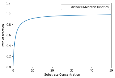
That’s a pretty classic illustration of a catalytic reaction that starts off in a positive order regime where rate increases with substrate concentration and then becomes independent of substrate concentration (zero order). That region where rate is zero order in substrate concentration is indicative of “saturation kinetics.” This basically means that all of the free enzyme is bound to substrate, so none is left to bind more substrate. As a consequence, adding more substrate does not increase the rate of reaction.
I find this very easy to see if I go back to the analytical solution for the concentration of the Enzyme Substrate Complex:
And the free enzyme concentration:
If we substitute the second into the first, we find (note that I replaced the messy fraction with 1/KM):
Factoring out the (1/KM) term before [S] in the denominator, we get a cancellation and are left with the following expression:
When the substrate concentration is low (\([S] \rightarrow 0\)), then \(K_M >> [S]\), and we find:
When the substrate concentration is hight (\([S] \rightarrow \infty\)), then \(K_M << [S]\), and we find:
Remember: the rate of this reaction is fundamentally given by \(r = k_2[ES]\). At low concentrations of substrate, we can see that adding more substrate increases the concentration of [ES] and so increases the rate of reaction. Once the substrate concentration gets high enough, though, we find ourselves in the position where all of the enzyme is bound to substrate, so we have basically exhausted all of the enzyme. Adding more does nothing to increase the rate because we have saturated the available enzyme under these conditions.